This paper aims to introduce the application of deep learning in the four basic tasks of computer vision, including classification (Figure a), positioning, detection (Figure b), semantic segmentation (Figure c), and instance segmentation (Figure d).
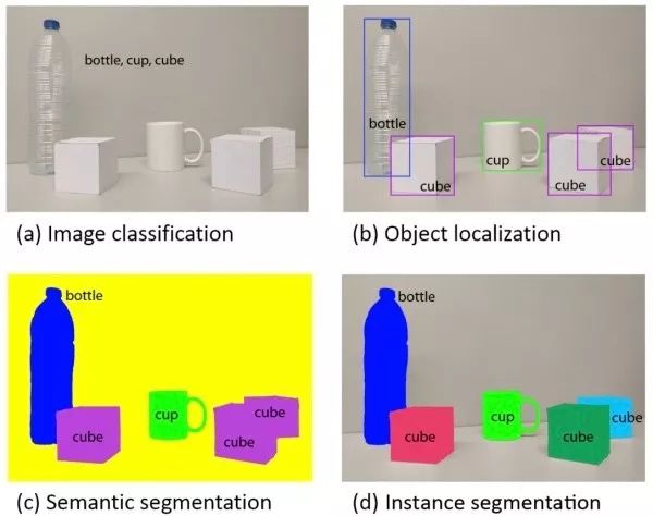
Image classification
Given an input image, the image classification task is designed to determine the category to which the image belongs.
(1) Image classification common data set
The following are several commonly used classification data sets, with increasing difficulty. Http://rodrigob.github.io/are_we_there_yet/build/ lists the performance rankings of each algorithm on each dataset.
MNIST 60k training image, 10k test image, 10 categories, image size 1 × 28 × 28, content is 0-9 handwritten numbers.
CIFAR-10 50k training image, 10k test image, 10 categories, image size 3 × 32 × 32.
CIFAR-100 50k training image, 10k test image, 100 categories, image size 3 × 32 × 32.
ImageNet 1.2M training images, 50k verification images, 1k categories. In 2017 and before, the ILSVRC competition based on ImageNet dataset will be held every year, which is equivalent to the computer vision world Olympics.
(2) Image classification classic network structure
Basic Architecture We use conv for the convolutional layer, bn for the bulk layer, and pool for the confluence layer. The most common network structure order is conv -> bn -> relu -> pool, where the convolutional layer is used to extract features and the confluence layer is used to reduce the size of the space. As the depth of the network progresses, the size of the image space will become smaller and smaller, and the number of channels will become larger and larger.
How to design a network for your mission? When faced with your actual task, if your goal is to solve the task instead of inventing a new algorithm, then don't try to design a new network structure yourself, and don't try to reproduce the existing network structure from zero. Look for the already implemented implementation and pre-training models for fine-tuning. Remove the last fully connected layer and the corresponding softmax, plus the fully connected layer and softmax for your task, then fix the previous layer and train only the parts you added. If you have more training data, you can fine-tune several layers and even fine-tune all layers.
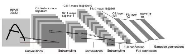
LeNet-560k parameters. The basic network architecture is: conv1 (6) -> pool1 -> conv2 (16) -> pool2 -> fc3 (120) -> fc4 (84) -> fc5 (10) -> softmax. The number in parentheses represents the number of channels, and 5 in the network name indicates that it has 5 layers of conv/fc layers. At the time, LeNet-5 was successfully used in ATMs to identify handwritten digits in checks. LeNet is named after its author's last name, LeCun.
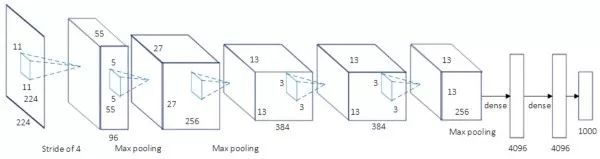
AlexNet 60M parameters, the champion network of ILSVRC 2012. The basic network architecture is: conv1 (96) -> pool1 -> conv2 (256) -> pool2 -> conv3 (384) -> conv4 (384) -> conv5 (256) -> pool5 -> fc6 (4096) -> Fc7 (4096) -> fc8 (1000) -> softmax. AlexNet has a similar network structure to LeNet-5, but with deeper and more parameters. Conv1 uses an 11×11 filter with a step size of 4 to quickly reduce the size of the space (227 × 227 -> 55 × 55). The key points of AlexNet are: (1). The ReLU activation function is used to make it have better gradient characteristics and faster training. (2). Random dropout is used. (3). Use data expansion technology in large quantities. The significance of AlexNet is that it won the ILSVRC competition in the same year with a performance of 10% higher than the second place, which makes people realize the advantages of the roll machine neural network. In addition, AlexNet also made people realize that they can use GPU to accelerate convolutional neural network training. AlexNet is named after its author Alex.
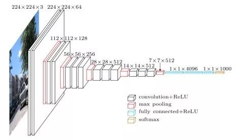
VGG-16/VGG-19 138M parameters, the runner-up network of ILSVRC 2014. The basic architecture of VGG-16 is: conv1^2 (64) -> pool1 -> conv2^2 (128) -> pool2 -> conv3^3 (256) -> pool3 -> conv4^3 (512) -> pool4 -> conv5^3 (512) -> pool5 -> fc6 (4096) -> fc7 (4096) -> fc8 (1000) -> softmax. ^3 stands for 3 repetitions. The key points of the VGG network are: (1). The structure is simple, only 3×3 convolution and 2×2 confluence configurations, and the same module combination is repeatedly stacked. The convolution layer does not change the size of the space, and the space size is halved each time the confluence layer is passed. (2). The amount of parameters is large, and most of the parameters are concentrated in the fully connected layer. 16 in the network name indicates that it has a 16-layer conv/fc layer. (3). Proper network initialization and the use of the batch normalization layer are important for training deep networks. The VGG-19 structure is similar to VGG-16 and has slightly better performance than VGG-16, but VGG-19 needs to consume more resources, so VGG-16 is actually used more. Since the VGG-16 network structure is very simple and suitable for migration learning, VGG-16 is still widely used. VGG-16 and VGG-19 are named after the author's research group name (Visual Geometry Group).
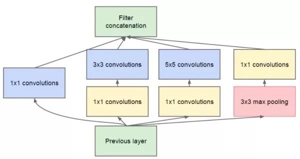
GoogLeNet 5M parameters, the champion network of ILSVRC 2014. GoogLeNet tries to answer the convolution of how large it should be when designing the network, or should choose the confluence layer. It proposes the Inception module, which uses 1 × 1, 3 × 3, 5 × 5 convolution and 3 × 3 confluence, and retains all results. The basic network architecture is: conv1 (64) -> pool1 -> conv2^2 (64, 192) -> pool2 -> inc3 (256, 480) -> pool3 -> inc4^5 (512, 512, 512, 528, 832) -> pool4 -> inc5^2 (832, 1024) -> pool5 -> fc (1000). The key points of GoogLeNet are: (1). Multi-branch processing separately, and cascading results. (2). In order to reduce the amount of calculation, a 1×1 convolutional dimension reduction is used. GoogLeNet uses a global average convergence instead of a fully connected layer to dramatically reduce network parameters. GoogLeNet is named after the author's unit (Google), where L is written to pay tribute to LeNet, and Inception's name comes from the "we need to go deeper" stalk in the Pirates of Dreams space.
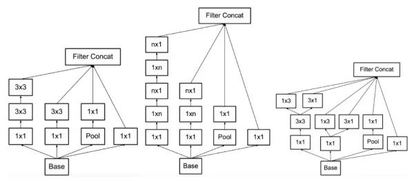
Inception v3/v4 further reduces the parameters based on GoogLeNet. It has a similar Inception module as GoogLeNet, but solves the 7×7 and 5×5 volume integrals into several equivalent 3×3 convolutions, and solves the 3×3 volume integrals into 1×3 and 3 in the back part of the network. ×1 convolution. This allows the network to be deployed to layer 42 with similar network parameters. In addition, Inception v3 uses a batch to layer one layer. Inception v3 is 2.5 times the amount of GoogLeNet calculations, and the error rate is 3% lower than the latter. Inception v4 combines the residual module (see below) with the Inception module to further reduce the error rate by 0.4%.
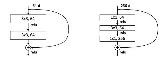
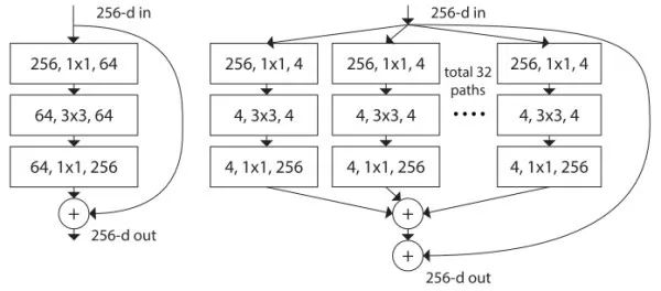
ResNet ILSVRC 2015 champion network. ResNet aims to solve the problem of increased training difficulty after the network is deepened. It proposes a residual module that contains two 3×3 convolutions and a short-circuit connection (left). The short-circuit connection can effectively alleviate the gradient disappearance caused by the deep depth when back propagation, which makes the performance of the network not deteriorate after deepening. Short-circuit connection is another important idea of ​​deep learning. In addition to computer vision, short-circuit connections are also used in machine translation, speech recognition/synthesis. In addition, ResNet with short-circuit connections can be seen as an integration of networks with many different depths and shared parameters, with the number of networks increasing with the number of layers. The key points of ResNet are: (1). Using short-circuit connections makes it easier to train deep layers and repeat the same stack of modules. (2). ResNet uses a large number of batches. (3). For deep networks (more than 50 layers), ResNet uses a more efficient bottleneck structure (right below). ResNet has achieved more than one person's accuracy on ImageNet.
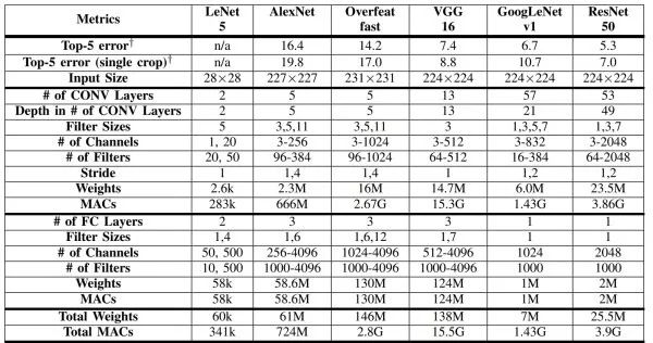
The table below compares the above several network structures.
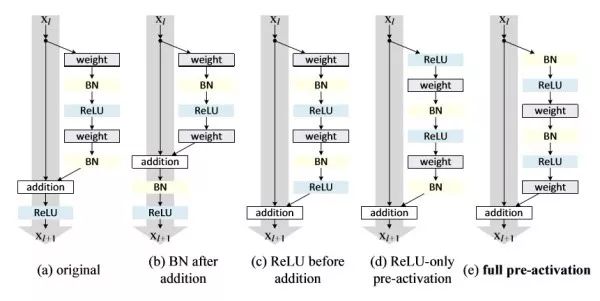
Improvements to preResNet ResNet. preResNet completes the order of the layers in the residual module. Compared with the classic residual module (a), (b) sharing BN will affect the short-circuit propagation of information, making the network more difficult to train and performance worse; (c) directly moving ReLU to BN will make the output of the branch Always non-negative, the network representation ability is reduced; (d) ReLU solves the non-negative problem of (e) in advance, but ReLU cannot enjoy the effect of BN; (e) ReLU and BN are solved in advance (d) . The short-circuit connection (e) of preResNet can transmit information more directly, and thus achieve better performance than ResNet.
Another improvement in ResNeXt ResNet. The traditional approach is usually to deepen or widen the network to improve performance, but the computational overhead will also increase. ResNeXt is designed to improve performance without changing the complexity of the model. Inspired by the streamlined and efficient Inception module, ResNeXt turns the non-short-circuit branch of ResNet into multiple branches. Unlike Inception, each branch has the same structure. The key points of ResNeXt are: (1). Follow the short-circuit connection of ResNet and repeat stacking the same module combination. (2). Multi-branch processing separately. (3). Use 1 × 1 convolution to reduce the amount of calculation. It combines the advantages of ResNet and Inception. In addition, ResNeXt is cleverly implemented using packet convolution. ResNeXt found that increasing the number of branches is a more effective way to improve network performance than deepening or widening. The naming of ResNeXt is intended to show that this is the next generation (next) ResNet.
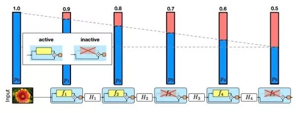
Random depth Improvements in ResNet. Designed to ease gradient disappearance and accelerate training. Similar to random dropout, it inactivates the residual module at random with a certain probability. The deactivated module is output directly from the short-circuit branch without passing through the parameterized branch. Feed forwards through all modules during testing. The random depth indicates that the residual module is information redundant.
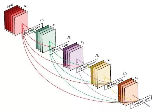
The purpose of DenseNet is also to avoid the gradient disappearing. Unlike the residual module, there is a short-circuit connection between any two layers in the dense module. That is to say, the input of each layer contains the results of all previous layers by concatenation, that is, the features of all levels from low to high. Unlike the previous method, the number of filters in the convolutional layer in DenseNet is small. DenseNet can achieve ResNet performance with only half of ResNet's parameters. In terms of implementation, the authors pointed out in the conference report that direct output cascading would take up a lot of GPU storage. Later, through shared storage, deeper DenseNet can be trained under the same GPU storage resources. However, because some intermediate results require repeated calculations, this implementation increases training time.
Object localization
Based on image classification, we also want to know where the target in the image is specific to the image, usually in the form of a bounding box.
The basic idea
Multitasking, the network has two output branches. One branch is used for image classification, that is, full connection + softmax to determine the target category, and the difference between simple image classification is that a "background" class is additionally needed here. The other branch is used to determine the target position, that is, the completion of the regression task outputs four digital mark bounding box positions (for example, the center point horizontal and vertical coordinates and the bounding box length and width), and the branch output result is only when the classification branch judges not to be "background" Only use.
Human body posture positioning / face positioning
The idea of ​​target positioning can also be used for human pose positioning or face positioning. Both of these require us to return to a series of human joints or face key points.
Weak supervision and positioning
Since target location is a relatively simple task, the recent research hotspot is to target the target only under the condition of tag information. The basic idea is to find some high-response saliency areas from the convolution results, and think that this area corresponds to the target in the image.
Object detection
In target positioning, there is usually only one or a fixed number of targets, and target detection is more general, and the types and numbers of targets appearing in the image are not fixed. Therefore, target detection is a more challenging task than targeting.
(1) Target detection common data set
The PASCAL VOC contains 20 categories. The trainval union of VOC07 and VOC12 is usually used as a training, and the test set of VOC07 is used as a test.
MS COCO COCO is more difficult than VOC. The COCO contains an 80k training image, a 40k verification image, and a 20k test-dev without a public mark, 80 categories, with an average of 7.2 targets per chart. The union of 80k training and 35k verification images is usually used as training, the remaining 5k images are used for verification, and the 20k test images are used for online testing.
mAP (mean average precision) Common evaluation indicators in target detection, calculated as follows. The prediction is considered correct when the ratio of the predicted bounding box to the real bounding box is greater than a certain threshold (usually 0.5). For each category, we plot its precision-precision-recall curve, and the average accuracy is the area under the curve. Then average the average accuracy of all categories to get mAP, which takes [0, 100%].
The area of ​​the intersection of the bounding box and the real bounding box predicted by the intersection over union (IoU) algorithm is divided by the area of ​​the union of the two bounding boxes, and the value is [0, 1]. The intersection ratio measures the proximity of the bounding box predicted by the algorithm and the real bounding box. The larger the cross ratio, the higher the degree of overlap between the two bounding boxes.
(2) Target detection algorithm based on candidate regions
The basic idea
Use different sized windows to slide across the image, and in each area, target the area within the window. That is, the area feedforward network within each window, its classification branch is used to determine the category of the area, and the regression branch is used to output the bounding box. The motivation for target detection based on sliding windows is that although the original image may contain multiple targets, there is usually only one target (or none) in the local area of ​​the image corresponding to the sliding window. Therefore, we can use the idea of ​​target positioning to process the areas within the window one by one. However, since this method has to slide all areas of the image once, and the size of the sliding window is different, this will bring a lot of computational overhead.
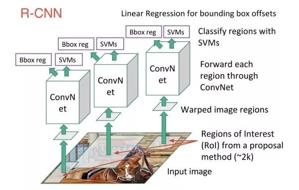
R-CNN
First use some non-deep learning class-independent unsupervised methods to find some candidate regions in the image that may contain targets. Then, for each candidate region feedforward network, target positioning, that is, two branches (classification + regression) output is performed. Among them, we still need to regress the branch because the candidate region is only a rough estimate of the target region. We need to use the regression branch to obtain more accurate bounding box prediction results. The importance of R-CNN is that the target detection is close to the bottleneck period, and R-CNN is good at improving the mAP on VOC from 35.1% to 53.7% in the method of fine-tuning the ImageNet pre-training model, which determines the basics of target detection under deep learning. Ideas. One interesting point is that the first sentence of the R-CNN paper has only two words "Features matter." This is the core of the deep learning method.
Candidate region (region proposal)
The candidate region generation algorithm usually combines similar pixels based on the color, texture, area, position, etc. of the image, and finally a series of candidate matrix regions can be obtained. These algorithms, such as selective search or EdgeBoxes, usually only take a few seconds of CPU time, and a typical number of candidate regions is 2k. The candidate region-based approach is very efficient compared to sliding all regions of the image with a sliding window. . On the other hand, the precision of these candidate region generation algorithms is general, but the recall is usually high, which makes it difficult for us to miss the target in the image.
Fast R-CNN
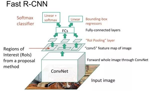
The drawback of R-CNN is that it requires multiple feedforward networks, which makes R-CNN inefficient, and it takes 47 seconds to predict an image. Fast R-CNN is also based on candidate regions for target detection, but inspired by SPPNet, in Fast R-CNN, the convolution feature extraction portions of different candidate regions are shared. That is to say, we first feed the entire image to the network and extract the conv5 convolution feature. Then, based on the result of the candidate region generation algorithm, the convolution feature is sampled, and this step is called convergence of interest regions. Finally, for each candidate region, target positioning is performed, that is, two branches (classification + regression) output.
Region of interest pooling, RoI pooling
The convergence of interest regions is intended to extract fixed-size features from local convolution features corresponding to candidate regions of arbitrary size, because the next two-branch network requires a fixed input size due to the fully connected layer. The method is to first project the candidate region onto the convolution feature, and then spatially divide the corresponding convolution feature region into a fixed number of grids (the number is determined according to the desired input size of the next network, for example, VGGNet needs 7×7 Grid), and finally the maximum convergence in each small grid area to get a fixed size convergence result. Consistent with the classic maximum convergence, the convergence of the regions of interest for each channel is independent.
Faster R-CNN
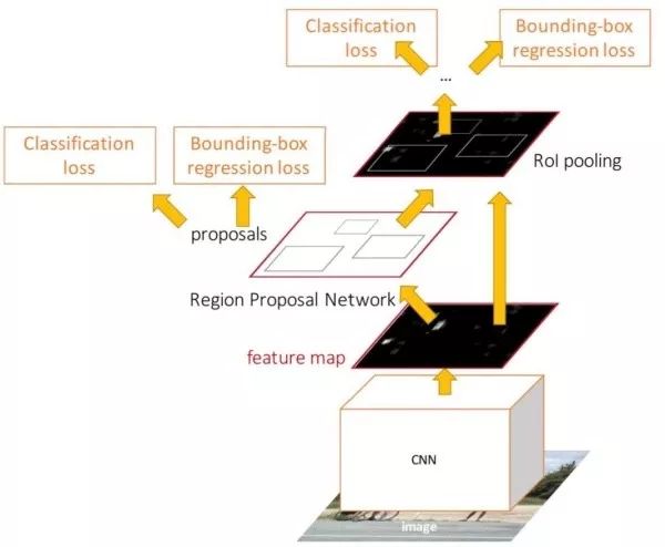
In the Fast R-CNN test, each image feedforward network takes only 0.2 seconds, but the bottleneck is that it takes 2 seconds to extract the candidate area. The Faster R-CNN no longer uses the existing unsupervised candidate region generation algorithm, but uses the candidate region network to generate candidate regions from the conv5 feature and integrates the candidate region network into the end-to-end training throughout the network. The Faster R-CNN test time is 0.2 seconds, which is close to real time. Later studies have found that by using fewer candidate areas, it is possible to further speed up under the condition that performance loss is small.
The region proposal networks (RPN) output two branches on the convolution feature by two-layer convolution (3×3 and 1×1 convolution). One branch is used to determine whether each anchor box contains a target, and the other branch outputs 4 coordinates of the candidate area for each anchor box. The candidate area network actually continues the idea of ​​target positioning based on the sliding window, except that the candidate area network slides on the convolution feature instead of the original picture. Since the space size of the convolution feature is small and the receptive field is large, even if a 3×3 sliding window is used, it can correspond to a large original image area. Faster R-CNN actually uses 3 sets of sizes (128×128, 256×256, 512×512), 3 sets of aspect ratio (1:1, 1:2, 2:1), a total of 9 anchor boxes, here The size of the anchor box has exceeded the size of the conv5 feature receptive field. For a 1000×600 image, 20k anchor boxes can be obtained.
Why use an anchor box?
The anchor box is a bounding box of predefined shape and size. Reasons for using the anchor box include: (1). The size of the candidate area in the image is different from the aspect ratio, and the direct regression is more difficult to train than the anchor box coordinate correction. (2). The conv5 feature receptive field is very large. It is very likely that the receptive field contains more than one target. Multiple anchor boxes can be used to predict multiple targets in the receptive field at the same time. (3). The use of anchor boxes can also be considered as a way to introduce prior knowledge into neural networks. We can set a set of anchor boxes based on the shape and size that the bounding box usually appears in the data. The anchor boxes are independent, and different anchor boxes correspond to different targets. For example, a tall and thin anchor box corresponds to a person, and a chunky anchor box corresponds to a vehicle.
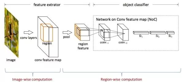
R-FCN
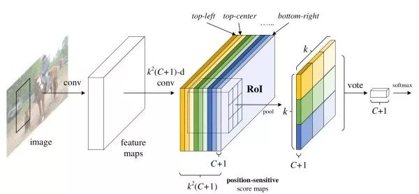
After the RoI pooling, the Faster R-CNN needs to perform two-branch prediction separately for each candidate region. R-FCN is designed to enable almost all computing sharing to further speed up. Since the image classification task does not care about the location of the target specific to the image, the network has translation invariance. However, in the target detection, because the position of the target is to be returned, the network output should be affected by the target translation. In order to alleviate the contradiction between the two, the R-FCN explicitly gives the depth convolution feature each channel in a positional relationship. When the RoI merges, the candidate region is first divided into 3×3 meshes, then different meshes are corresponding to different channels of the candidate convolution feature, and finally each mesh is averagely merged. R-FCN also uses two branches (classification + regression) output.
summary
Target detection algorithms based on candidate regions usually require two steps: the first step is to extract depth features from the image, and the second step is to locate each candidate region (including classification and regression). The first step is image level calculation. One image only needs to feed the part of the network once, and the second step is the area level calculation. Each candidate area needs to feed the part network once. Therefore, the second step takes up the overall main computational overhead. The evolution of R-CNN, Fast R-CNN, Faster R-CNN, and R-FCN algorithms is to gradually increase the proportion of image-level calculations in the network while reducing the proportion of regional-level calculations. Almost all calculations in R-CNN are region-level calculations, and almost all calculations in R-FCN are image-level calculations.
(3) Target detection algorithm based on direct regression
The basic idea
The candidate region-based method has two steps, although the detection performance is better, there are still some gaps in speed from real-time. The method based on direct regression does not require candidate regions and directly outputs classification/regression results. This type of method can achieve real-time speed because the image only needs to feed the network once.
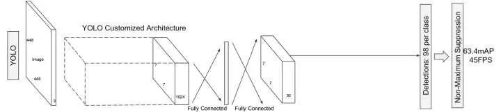
YOLO
The image is divided into a 7×7 grid in which the real target in the image is divided by it into the grid where the target center is located and its closest anchor box. For each grid area, the network needs to predict: the probability that each anchor box contains the target (0 should be included when the target is not included, otherwise it is the IoU of the anchor box and the real bounding box), the 4 coordinates of each anchor box, The class probability distribution of the grid. The class probability distribution for each anchor box is equal to the probability that each anchor box contains the target multiplied by the class probability distribution for that grid. Compared to the candidate region-based approach, YOLO needs to predict the probability of including the target because most of the regions in the image do not contain targets, and the coordinates and category probability distributions are updated only when the target exists during training.
The advantages of YOLO are: (1). The receptive field of the candidate region-based method is a local region in the image, and YOLO can utilize the information of the entire image. (2). Have better generalization ability.
The limitations of YOLO are: (1). It is not well handled when the number of targets in the grid exceeds a preset fixed value, or if multiple targets in the grid belong to one anchor box at the same time. (2). The ability to detect small targets is not good enough. (3). The detection ability of the bounding box of the uncommon aspect ratio is not strong. (4). The bounding box size is not considered when calculating the loss. Small offsets in large bounding boxes and small offsets in small bounding boxes should have different effects.
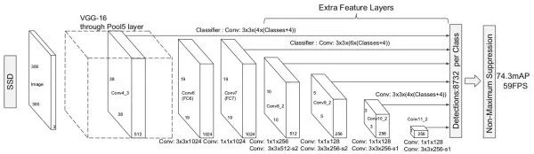
SSD
Compared with YOLO, SSD adds several convolution layers after the convolution feature to reduce the feature space size, and detects the targets of different sizes by combining the detection results of the multi-layer convolution layer. In addition, similar to the RPN of Faster R-CNN, the SSD replaces the fully connected layer in YOLO with a 3x3 convolution to classify/regress the anchor boxes of different sizes and aspect ratios. The SSD is faster than YOLO and is close to the detection performance of Faster R-CNN. Later studies have found that SSDs are relatively less affected by the performance of the underlying model than other methods.
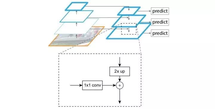
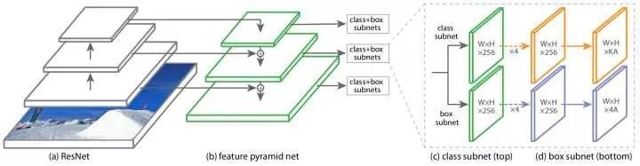
FPN
Previous methods have taken high-level convolution features. However, because high-level features will lose some details, FPN combines multiple layers of features to enhance high-level, low-resolution, strong semantic information and low-level, high-resolution, and weak semantic information to enhance the network's ability to handle small targets. In addition, unlike the method of making predictions using the results of multi-layer fusion, FPN is independently predicted at different layers. FPN can be combined with candidate region based methods or with direct regression based methods. After the FPN is combined with the Faster R-CNN, the detection performance of the small target is greatly improved without substantially increasing the calculation amount of the original model.
RetinaNet
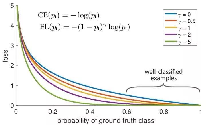
RetinaNet believes that the method based on direct regression is usually not as good as the candidate region based approach, because the former faces extreme category imbalances. The candidate region-based approach can filter out most of the background region through the candidate region, but the method based on direct regression needs to directly face the category imbalance. Therefore, RetinaNet proposes a focal loss function by improving the classic cross entropy loss to reduce the loss value of a good sample that has already been scored, so that the model training is more concerned with difficult examples. RetinaNet has achieved near-speed based on direct regression methods, and performance beyond the candidate region-based approach.
(4) Common techniques for target detection
Non-max suppression (NMS)
One problem that may arise with target detection is that the model makes multiple predictions for the same target, resulting in multiple bounding boxes. The NMS aims to preserve the prediction that is closest to the real bounding box and suppress other predictions. The NMS approach is, first, for each category, the NMS first counts the probability of the category output for each prediction result, and ranks the prediction results from high to low. Secondly, the NMS believes that the prediction result with a small probability does not find the target, so it is suppressed. Then, in the remaining prediction results, the NMS finds the prediction result with the highest probability, outputs it, and suppresses other bounding boxes that have a large overlap with the bounding box (such as IoU greater than 0.3). Repeat the previous step until all predictions are processed.
Online hard example mining (OHEM)
Another problem with target detection is that the categories are not balanced. Most of the areas in the image do not contain targets, while only a small area contains targets. In addition, the difficulty of detecting different targets is also very different. Most of the targets are easily detected, while a small number of targets are very difficult. OHEM is similar to Boosting in that it sorts all candidate regions according to the loss value and selects some of the candidate regions with the highest loss value for optimization, so that the network pays more attention to the more difficult targets in the image. In addition, in order to avoid selecting candidate regions that overlap each other greatly, the OHEM performs NMS on the candidate regions according to the loss value.
Logarithmic space regression
Regression is much more difficult than classification optimization. L2\ell_ loss is sensitive to outliers. Because of the squaredness, the outliers will have large loss values, and there will be a large gradient, which makes gradient explosions easy to occur during training. The gradient of L1\el loss is not continuous. In the logarithmic space, since the dynamic range of the values ​​is much smaller, regression training is much easier. In addition, some people use the smooth L1\el loss to optimize. Pre-normalizing regression goals can also help with training.
Semantic segmentation
Semantic segmentation is a more advanced task of target detection. Target detection only needs to frame the bounding box of each target. Semantic segmentation needs to further determine which pixels in the image belong to which target.
(1) Semantic segmentation commonly used data sets
PASCAL VOC 2012 1.5k training image, 1.5k verification image, 20 categories (including background).
MS COCO COCO is more difficult than VOC. There are 83k training images, 41k verification images, 80k test images, and 80 categories.
(2) Basic ideas of semantic segmentation
The basic idea
Image classification is performed pixel by pixel. We input the whole image into the network, so that the output space size is consistent with the input. The number of channels is equal to the number of categories, which respectively represent the probability that each spatial position belongs to each category, that is, it can be classified pixel by pixel.
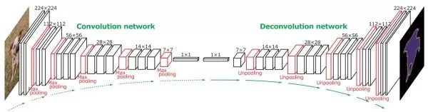
Full convolution network + deconvolution network
In order to make the output have a three-dimensional structure, there is no fully connected layer in the full convolutional network, only the convolutional layer and the confluent layer. However, as convolution and convergence progress, the number of image channels is getting larger and larger, and the size of the space is getting smaller and smaller. To make the output and input have the same amount of space, a full convolutional network needs to use deconvolution and anti-convergence to increase the size of the space.
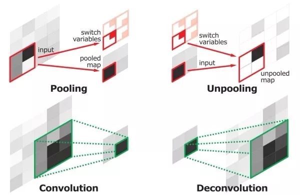
Deconvolution / transpose convolution
The standard convolution filter slides in the input image, multiplying each time the local region of the input image is multiplied to obtain an output, and the deconvolution filter is slid in the output image, each multiplied by an input neuron. The device gets an output local area. The forward process of deconvolution and the reverse process of convolution complete the same mathematical operations. Like the standard convolution filter, the deconvolution filter is also learned from the data.
Inverse maximal convergence (max-unpooling)
Generally, the full convolution network is a symmetrical structure. When the maximum convergence, it is necessary to record the local area position where the maximum value is located, and the corresponding position output is input as input when the corresponding inverse maximum convergence is performed, and the remaining positions are zero-padded. The inverse maximum convergence can compensate for the spatial information lost at the maximum confluence. The forward process of the inverse maximum convergence and the reverse process of the maximum convergence complete the same mathematical operation.
(3) Common techniques for semantic segmentation
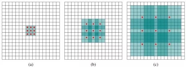
Dilated convolution
A technique often used to segment tasks to increase the effective receptive field. The input local area corresponding to each output neuron in the standard convolution operation is continuous, and the input local area corresponding to the expanded convolution is discontinuous in spatial position. The expansion convolution keeps the amount of convolution parameters constant, but has a larger effective receptive field.
Conditional random field (CRF)
A conditional random field is a probability map model that is often used to micro-repair the output of a full-convolution network to make the details better. The motivation is that pixels that are close in distance, or pixels with similar pixel values, are more likely to belong to the same category. In addition, research work uses recurrent neural networks to approximate conditional random fields. Another disadvantage of conditional random walks is that they consider the relationship between two or two pixels, which makes them inefficient.
Use low-level information
Comprehensive use of low-level results can make up for the details and edge information lost as the network deepens.
Instance segmentation
Semantic segmentation does not distinguish between different instances belonging to the same category. For example, when there are multiple cats in the image, semantic segmentation predicts all pixels of the two cats as "cat". In contrast, instance segmentation needs to distinguish which pixels belong to the first cat and which pixels belong to the second cat.
The basic idea
Target detection + semantic segmentation. First, use the target detection method to frame different instances in the image, and then use the semantic segmentation method to mark pixels by pixel in different bounding boxes.
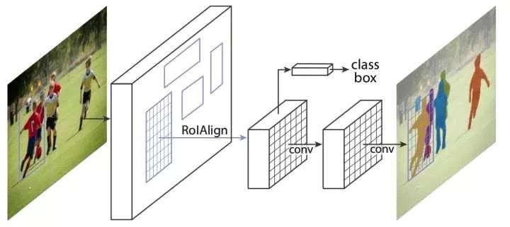
Mask R-CNN
Target detection is performed using FPN, and semantic segmentation is performed by adding additional branches (the extra split branch and the original detection branch do not share parameters), that is, the Master R-CNN has three output branches (classification, coordinate regression, and segmentation). In addition, other improvements of Mask R-CNN are: (1). Improved RoI convergence, the alignment of candidate regions and convolution features is not lost due to bilinear difference. (2). At the time of segmentation, Mask R-CNN decouples the two tasks of the judgment category and the output template (mask), and uses sigmoid with the logistic loss function to process each template separately, and obtains the ratio. The classic segmentation method uses softmax to make all categories compete for better results.
SHAOXING COLORBEE PLASTIC CO.,LTD , https://www.colorbeephoto.com