Decision trees are a very common classification method in machine learning, and can be said to be the most intuitive and best understood algorithm among all algorithms.
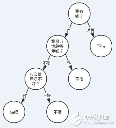
Someone is looking for me to borrow money (of course it is unlikely...), borrow or not? I will combine my three characteristics based on whether I have money, whether I use money or not, and my credit is good.
We turn to a more general perspective. For some characteristic data, if we can have such a decision tree, we can easily predict the conclusion of the sample. So the question is translated into how to find a suitable decision tree, that is, how to sort these features.
Imagine before sorting features. When making a decision on a feature, we definitely hope that the higher the purity of the sample after classification, the better, that is, the samples of the branch nodes belong to the same category as much as possible.
So when choosing the root node, we should choose the feature that will make the "branched node the most pure". After processing the root node, for its branch nodes, the idea of ​​continuing to apply the root node is recursively, so that a tree can be formed. This is actually the basic idea of ​​greedy algorithms. So how do you quantify the "highest purity"? Entropy is what it is, it is our most commonly used measure of purity. Its mathematical expression is as follows:
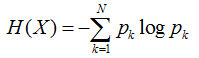
Where N is the number of possible values ​​for the conclusion, and p is the probability of occurrence when taking the kth value, which is the frequency/total number of occurrences for the sample.
The smaller the entropy, the purer the sample.
The function image of the entropy of a two-point distribution sample X (x = 0 or 1) is illustrated. The abscissa indicates the probability that the sample value is 1, and the ordinate indicates the entropy.
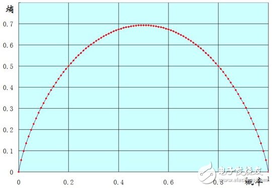
It can be seen that when p(x=1)=0, that is to say all samples are 0, the entropy is 0.
When p(x=1)=1, that is to say all samples are 1 and the entropy is also 0.
When p(x=1)=0.5, that is, 0,1 in the sample each account for half, and the entropy can obtain the maximum value.
To expand, sample X may take the value n (x1....xn). It can be proved that when p(xi) is equal to 1/n, that is, the sample is absolutely uniform and the entropy can reach the maximum. When p(xi) has a value of 1, all others are 0, that is, the sample value is xi, and the entropy is the smallest.
Decision tree algorithmID3
Assume that in sample set X, for a feature a, it may have (a1, a2, .an) these values. If the feature set A is used to divide the sample set X (put it as the root node), there will definitely be n Branch nodes. As I mentioned earlier, we hope that after the division, the sample of the branch node is as pure as possible, that is, the "total entropy" of the branch node is as small as possible.
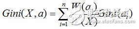
Because the number of nodes in each branch is different, we should make a weight when calculating the "total entropy", assuming that the number of samples of the i-th node is W(ai), and its weight in all samples is W. (ai) / W(X). So we can get a total entropy:
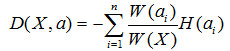
This formula represents the meaning of a sentence: the sum of the entropies of the individual nodes after weighting. The smaller the value, the higher the purity.
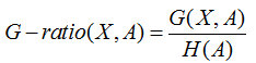
At this time, we introduce a noun called information gain G(X, a), which means that the feature of a brings the information to the sample. The formula is: ![]() Since H(X) is a fixed value for one sample, the information gain G should be as large as possible. Finding the feature that maximizes the information gain as the target node and gradually recursively constructing the tree is the idea of ​​the ID3 algorithm. Let's take a simple example to illustrate the calculation of the information gain:
Since H(X) is a fixed value for one sample, the information gain G should be as large as possible. Finding the feature that maximizes the information gain as the target node and gradually recursively constructing the tree is the idea of ​​the ID3 algorithm. Let's take a simple example to illustrate the calculation of the information gain:
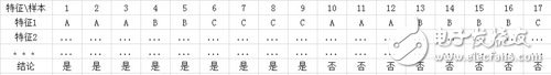
In the above example, I calculate the information gain of feature 1.
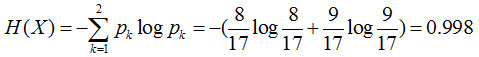
First calculate the entropy H(X) of the sample
After calculating the total entropy, we can see that feature 1 has 3 nodes A, B, and C, which are 6, 6, and 5, respectively.
So the weight of A is 6/(6+6+5), the weight of B is 6/(6+6+5), and the value of C is 5/(6+6+5).
Because we hope that the higher the purity of the node after the division, the better, so we need to calculate the entropy of nodes A, B, and C separately.
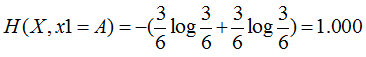
Feature 1=A: 3 yes, 3 no, its entropy is
Feature 1=B: 2 yes, 4 no, its entropy is

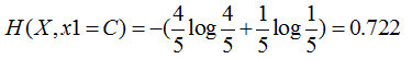
Feature 1=C: 4 yes, 1 no, its entropy is
The total entropy of such a branch node is equal to:
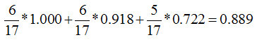
The information gain of feature 1 is equal to 0.998-0.889=0.109
Similarly, we can also calculate the information gain of Other features, and finally take the feature with the largest information gain as the root node.
The above calculations can also be derived from empirical conditional entropy: G(X, A) = H(X) - H(X|A), which can be understood by interested students.
C4.5
There is actually a very obvious problem in the ID3 algorithm.
If there is a sample set, it has a (unique) feature called id or name, and that's it. Imagine that if there are n samples, the id feature will definitely divide the sample into n parts, that is, there are n nodes, each node has only one value, and the entropy of each node is zero. That is to say, the total entropy of all branch nodes is 0, then the information gain of this feature will reach the maximum value. Therefore, if ID3 is used as the decision tree algorithm at this time, the root node must be the id feature. But obviously this is unreasonable. . .
Of course, the above is the limit case. In general, if a feature is too sparse for the sample partition, this is also unreasonable (in other words, the feature that favors more values). To solve this problem, the C4.5 algorithm uses the information gain rate as the feature selection criterion.
The so-called information gain rate is based on the information gain, except for a split informaTIon, to punish more attributes.
And this split informaTIon is actually the entropy H(A) of the number of features.
Why can this be reduced? Let's understand it with the example of id above. If id divides n samples into n parts, then the probability of the value of id is 1/n. The article has already said that when the sample is absolutely uniform, the entropy is the largest.
Therefore, this case is characterized by id. Although the information gain is the largest, the penalty factor split informaTIon is also the largest, so as to lower its gain rate, which is the idea of ​​C4.5.
CART
The purpose of the decision tree is ultimately to find a quantitative standard that distinguishes the purity of the sample. In the CART decision tree, the Gini index is used as its metric. The intuitive understanding of the Gini coefficient is that two samples are randomly extracted from the set. If the sample set is purer, the probability of taking different samples is smaller. This probability reflects the Gini coefficient.
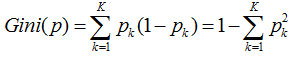
So if a sample has K classifications. Assuming that a certain feature a of a sample has n values, the probability that one of the nodes takes a different sample is: ![]()
So the sum of the probabilities of the k categories, we call the Gini coefficient:
The Gini index is a weighting of the Gini coefficients of all nodes.
After calculation, we will select the feature with the smallest Gini coefficient as the optimal partitioning feature.
Pruning
The purpose of pruning is actually to prevent over-fitting, which is the most important means of preventing over-fitting in decision trees. In the decision tree, in order to train the sample as much as possible, our decision tree will continue to grow. However, sometimes training samples may be so good that they take the unique attributes of certain samples as general attributes. At this time we need to actively remove some branches to reduce the risk of overfitting.
There are two ways to pruning: pre-pruning and post-pruning.
Pre-pruning
In general, the tree will stop growing as long as the node sample is 100% pure. But this may have an overfitting, so we don't have to let it grow 100%, so before that, set some termination conditions to terminate it early. This is called pre-prune, and this process occurs before the decision tree is generated.
Generally, our means of pre-pruning are:
1. Limit the depth of the tree
2. The number of child nodes of the node is less than the threshold.
3. Set the threshold of the node entropy and so on.
Post pruning
As the name suggests, this pruning is after the decision tree is built. There are many algorithms for the post-prune algorithm, and some of them are quite esoteric. Here, I will not delve into the idea of ​​a simple algorithm.
Reduced-Error Pruning (REP)
The pruning method considers each node on the tree as a candidate for pruning, but there are some conditions that determine whether to pruning, usually with these steps:
1. Delete all its subtrees to make them leaf nodes.
2. Give the node the most relevant classification
3. Verify the accuracy with verification data and compare it before processing
If it is not worse than the original, it will actually delete its subtree. Then repeatedly handle the node from bottom to top. This approach is actually to deal with those "harmful" nodes.
Random forestThe theory of random forests should not be involved with the decision tree itself. Decision trees can only be used as an algorithm of their ideas.
Why introduce random forests? We know that we can only produce one decision tree for the same batch of data, and this change is relatively simple. Also have to use a combination of multiple algorithms?
This has the concept of integrated learning.
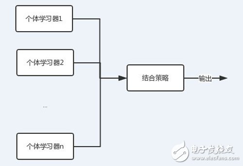
As can be seen in the figure, each individual learner (weak learner) can contain an algorithm, and the algorithms can be the same or different. If they are the same, we call it homogeneous integration, and vice versa.
Random forest is a special case of integrated learning based on bagging strategy.
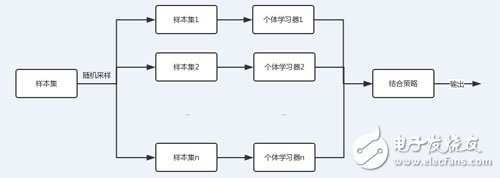
As can be seen from the above figure, the training set of the bagging individual learner is obtained by random sampling. With n random samples, we can get n sample sets. For the n sample sets, we can independently train n individual learners, and then use the set strategy to obtain the final output for the n individual learners. The n individual learners are independent of each other. Can be in parallel.
Note: There is another way to integrate learning called boosTIng. In this way, there is a strong correlation between learners, and those who are interested can understand.
The sampling method used in random forests is generally Bootstap sampling. For the original sample set, we randomly collect one sample into the sample set and put it back, which means that the sample may still be collected at the next sampling. After a certain number of samples, a sample set is obtained. Since it is random sampling, each time the sample set is different from the original sample set, and the other sample sets are different, the resulting individual learners are also different.
The main problem in the random forest is that there are n results, how to set the combination strategy, there are several main ways:
Weighted average method:
The averaging method is often used for regression. The practice is to have a pre-set weight wi for each learner.
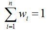
Then the final output is:
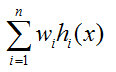
When the weight of the learner is 1/n, this averaging method is called the simple averaging method.
Voting method:
Voting is similar to voting in our lives, if the weight of each learner is the same.
Then there is an absolute voting method, that is, more than half of the votes. Relative to the voting method, the minority obeys the majority.
If there is weighting, it is still the minority to obey the majority, but the number inside is weighted.
example
Take a simple quadratic function code to see how the decision tree works.
The training data is 100 random real squared data, different depths will get different curves
The test data is also random data, but the models of trees of different depths produce different prediction values. As shown
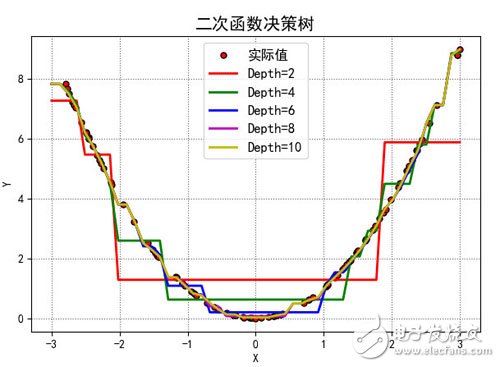
The code for this picture is as follows:
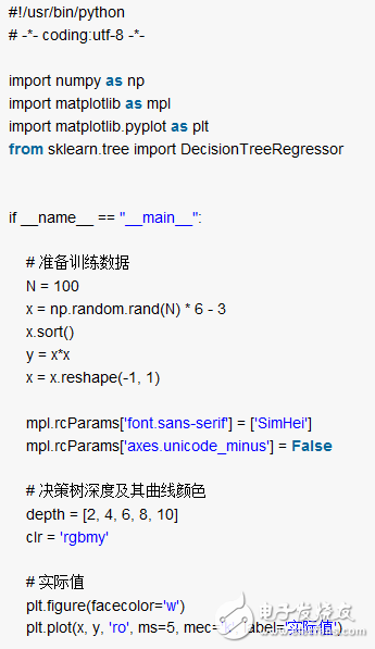
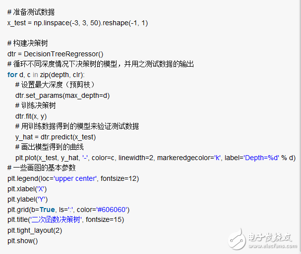
My python 3.6 environment, you need to install the three libraries numpy, matplotlib, sklearn, if necessary, directly pip install, you can run and see, although simple but very interesting.
Portable radios,Motorola Two Way Radios,Motorola Talkabout Radios,Motorola Handheld Radio
Guangzhou Etmy Technology Co., Ltd. , https://www.digitaltalkie.com