Deep learning basics
1 Basic concepts of deep learning
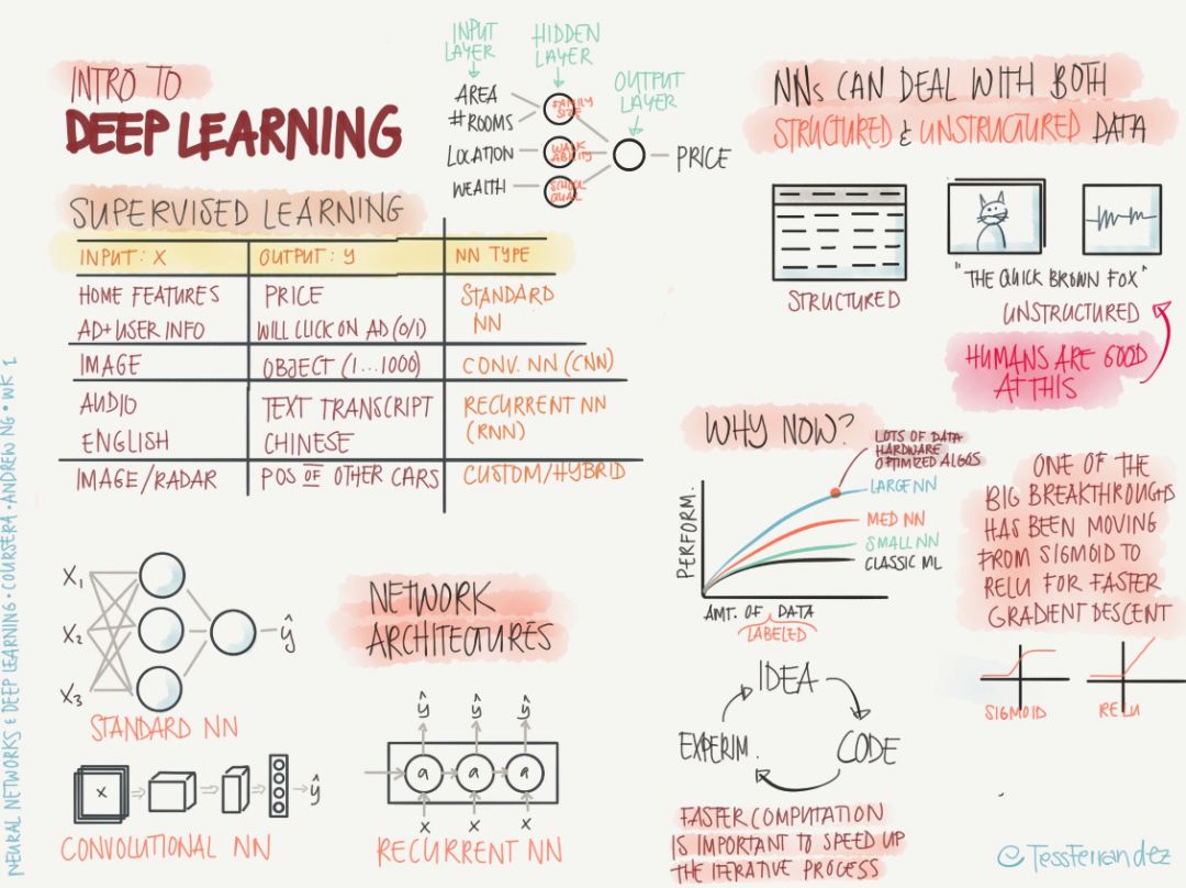
Supervised learning: All input data has definite corresponding output data. In various network architectures, the node layers of input data and output data are located at both ends of the network. The training process is to constantly adjust the weight of the network connection between them.
Top left: Lists the supervised learning of various network architectures. For example, a standard neural network (NN) can be used to train functions between house features and house prices. Convolutional neural networks (CNN) can be used to train images and categories. Function, Recurrent Neural Networks (RNN) can be used to train functions between speech and text.
Bottom left: Shows the simplified architecture of NN, CNN, and RNN, respectively. The forward processes of these three architectures are different. The NN uses the way in which the weight matrix (connection) and node values ​​are multiplied and propagated to the next layer of nodes one after the other; CNN uses rectangular convolution kernels to perform volumes on the image input in turn. Product operation, sliding, to get the next level of input; RNN remember or forget the information of previous time step to provide long-term memory for the current calculation process.
Top right: NN can handle structured data (tables, databases, etc.) and unstructured data (images, audio, etc.).
Bottom right: Deep learning can be developed mainly due to the emergence of big data. The training of neural networks requires a lot of data. Big data itself in turn promotes the emergence of larger networks. A major breakthrough in deep learning research is the emergence of new activation functions. Replacing a sigmoid function with a ReLU function can maintain a rapid gradient descent process in reciprocal propagation. The sigmoid function exhibits a zero derivative at positive infinity and negative infinity. This is the main reason why the gradient disappears, which results in slow training or even failure. To study deep learning, you need to learn the virtuous circle of "idea-code-experiment-idea".
2 logistic regression

Top left: Logistic regression is mainly used for binary problems. As shown in the figure, logistic regression can be used to solve whether an image is a cat problem. The image is input (x), and cat (1) or non-cat (0) is the output. . We can think of logistic regression as the problem of separating two sets of data points. If there is only linear regression (the activation function is linear), the data points for the non-linear boundary (for example, a group of data points is surrounded by another group) is Can not be effectively separated, so here we need to replace the linear activation function with a nonlinear activation function. In this case, we use the sigmoid activation function, which is a smooth function with a range of (0, 1), which allows the output of the neural network to get continuous, normalized (probability value) results, for example, when the output node is At (0.2, 0.8), it is determined that the image is non-cat (0).
Bottom left: The training goal of the neural network is to determine the most appropriate weight w and bias term b. What is the process like this?
This classification is actually an optimization problem. The purpose of the optimization process is to minimize the gap between the predicted value y hat and the real value y, which can be achieved formally by finding the minimum value of the objective function. Therefore, we first determine the form of the objective function (loss function, cost function), and then gradually update w, b with gradient descent. When the loss function reaches a minimum value or is small enough, we can obtain good prediction results.
Top right: A sketch of the change of the loss function value on the parametric surface. The gradient can be used to find the fastest falling path. The learning rate can determine the speed of convergence and the final result. When the learning rate is large, the initial convergence is rapid and it is difficult to stay at the local minimum, but it is difficult to converge to a stable value in the later period. When the learning rate is small, the situation is just the opposite. In general, we hope that the training rate at the beginning of training will be larger and the learning rate at the later stage will be smaller. Afterwards, the training methods for changing the learning rate will be introduced.
Bottom right: Summarizing the entire training process, starting from the input node x, the prediction output y hat is obtained by forward propagation, the loss function value is obtained by y hat and y, the back propagation is started, the w and b are updated, and the process is iterated repeatedly. Until convergence.
3 characteristics of shallow network
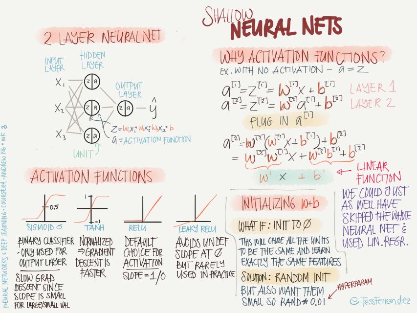
Top left: Shallow networks hide fewer layers. As shown in the figure, there is only one hidden layer.
Bottom left: Here are the characteristics of different activation functions:
The sigmoid:sigmoid function is often used for dichotomy problems, or the last layer of a multi-classification problem, mainly due to its normalized nature. The sigmoid function will tend to zero on both sides, which will result in slow training.
Tanh: The advantage of the tanh function relative to sigmoid is that the gradient value is larger, which can make the training faster.
ReLU: It can be understood as a threshold activation (a special case of spiking model, similar to the working of biological nerves). This function is very common and is basically the default selected activation function. The advantage is that it does not cause slow training, and because the activation value is zero. The nodes do not participate in back propagation and this function also has the effect of sparsifying the network.
Leaky ReLU: Avoiding the result of a zero-activation value makes the back-propagation process always executed, but it is rarely used in practice.
Top right: Why use an activation function? More precisely, why use a nonlinear activation function?
The example in the figure above shows that a neural network without an active function propagates through two layers. The final result is the same as a single-layer linear operation. That is, no matter how many layers are used, if no nonlinear activation function is used. The neural networks are all equivalent to a single neural network (without the input layer).
Bottom right: how to initialize the values ​​of parameters w, b?
When all parameters are initialized to zero, all nodes become the same, and only the same features can be learned during the training process, and multiple levels and diverse features cannot be learned. The solution is to randomly initialize all parameters, but only a small amount of variance is needed, so initialize with Rand(0.01), where 0.01 is also one of the hyperparameters.
4 Characteristics of deep neural networks

Top left: The parametric capacity of a neural network increases exponentially as the number of layers increases, that is, some deep neural networks can solve the problem. Shallow neural networks need relative finger count calculations to solve.
Bottom left: The deep network of CNN can combine the simple features of the bottom layer into more and more complex features. The greater the depth, the greater the complexity and diversity of the images that can be classified. The same is true of the deep network of RNNs, which can decompose speech into phonemes and then gradually compose letters, words, sentences and perform complex speech-to-text tasks.
Right: Depth network is characterized by a large amount of training data and computational resources. It involves a large number of matrix operations and can be executed on the GPU in parallel. It also contains a large number of hyperparameters, such as learning rate, number of iterations, number of hidden layers, and activation. Function selection, learning rate adjustment program, batch size, regularization method, etc.
5 Deviation and variance
What do you need to pay attention to when deploying your machine learning model? The following figure shows the problem of data set partitioning, deviations, and variances needed to build an ML application.
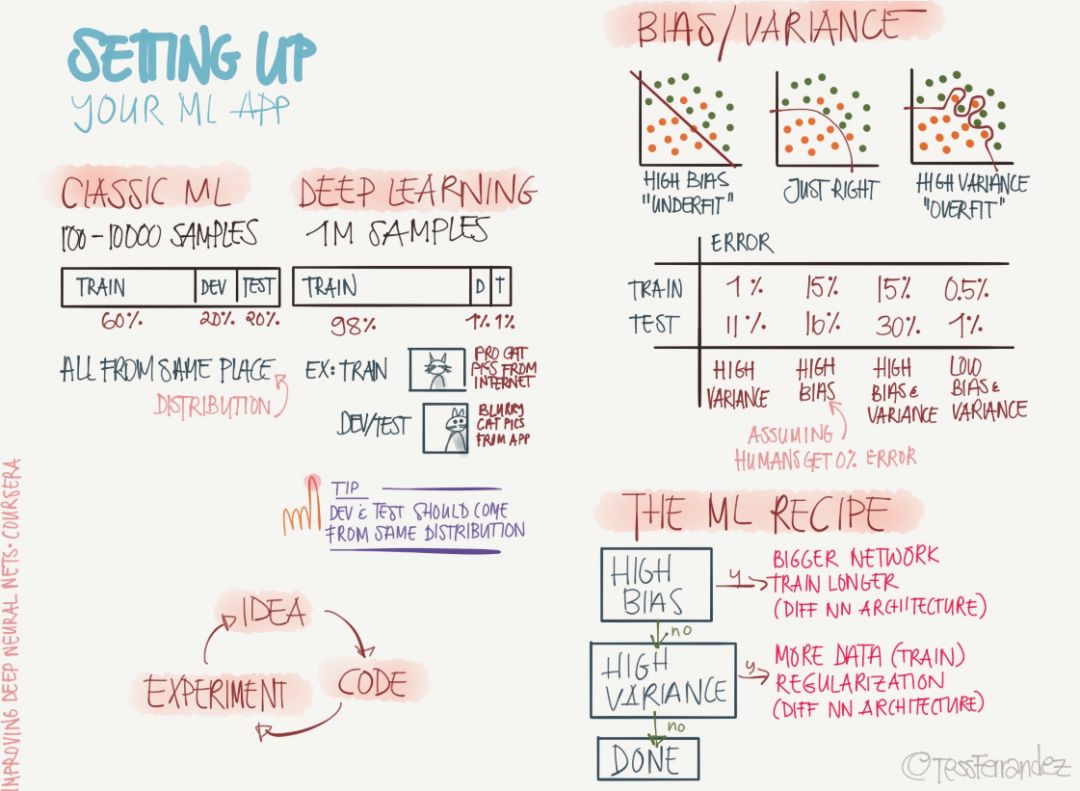
As shown above, the number of samples required for the classic machine learning and deep learning models is very different. The number of deep learning samples is thousands of times that of classical ML. Therefore, the distribution of training sets, development sets, and test sets is also very different. Of course, we assume that these different data sets obey the same distribution.
The problems of variance and variance are also common challenges in machine learning models. The above diagram shows the under-fitting due to high deviation and the over-fitting caused by high variance. In general, the problem of solving high deviations is to choose a more complex network or a different neural network architecture, while solving the high variance problem can add regularization, reduce model redundancy, or use more data for training.
Of course, the machine learning model needs to pay attention not only to these problems, but they are the most basic and important parts in configuring our ML applications. Others such as data preprocessing, data normalization, and the selection of hyperparameters are all reflected in the following information diagrams.
6 Regularization
Regularization is the main method to solve high variance or model overfitting. In the past few years, researchers have proposed and developed a variety of regularization methods suitable for machine learning algorithms, such as data enhancement, L2 regularization (weight attenuation), L1 regularity. , Dropout, Drop Connect, random pooling, and early termination.
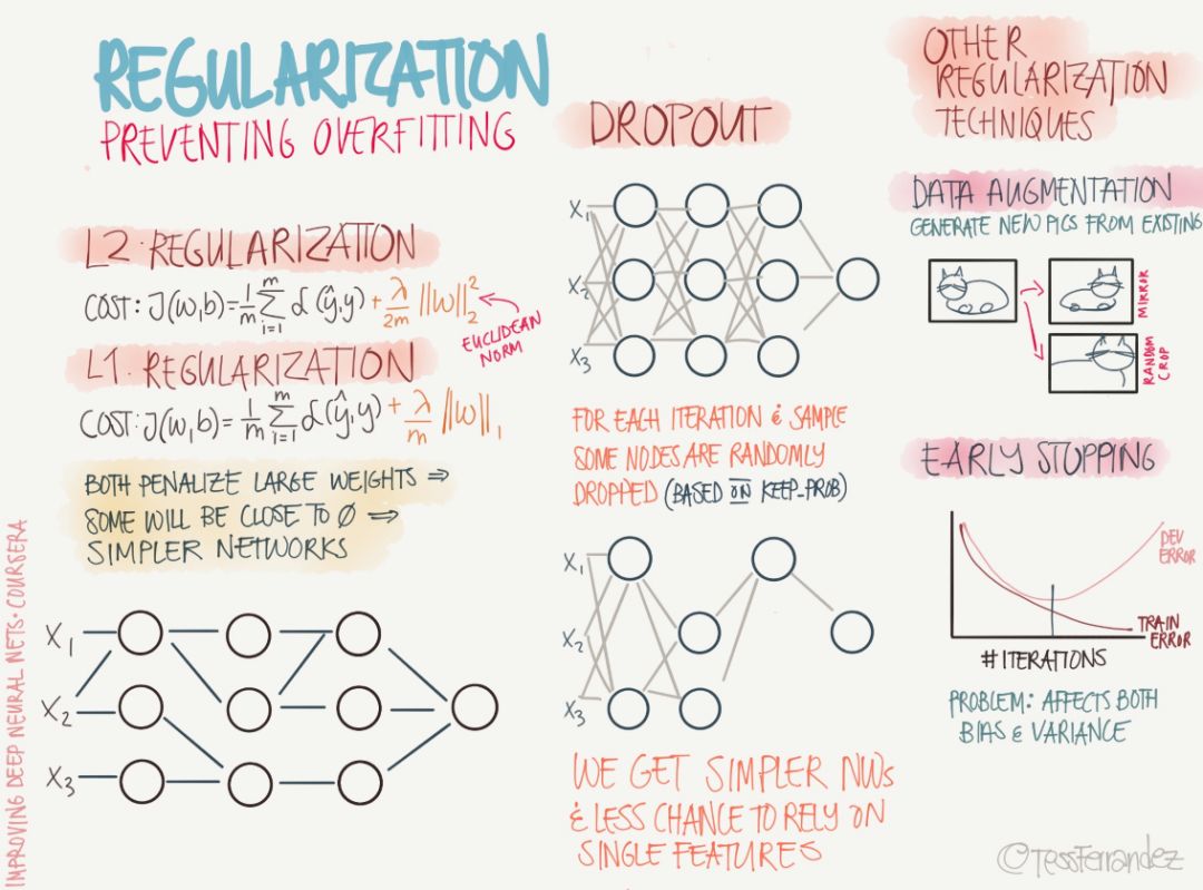
As shown in the left column above, L1 and L2 regularization are also the most widely used regularization methods in machine learning. L1 regularization adds a regularization term to the objective function to reduce the sum of the absolute values ​​of the parameters. In L2 regularization, the purpose of adding a regularization term is to reduce the sum of the parameter squares. According to previous studies, many parameter vectors in L1 regularization are sparse vectors because many models cause the parameters to approach zero, so it is often used in feature selection settings. In addition, the parameter norm penalty L2 regularization allows the deep learning algorithm to "perceive" to the input x with higher variance, so the feature weights with smaller (relatively increased variance) covariance with the output target will shrink.
In the middle column, the figure above shows the Dropout technique, which temporarily discards a subset of neurons and their connections. Randomly discarding neurons can prevent overfitting, while exponentially and efficiently connecting different network architectures. A neural network that generally uses Dropout technology sets a retention rate p, and each neuron randomly selects whether to remove it with a probability of 1-p in a batch of training. At the last inference, all neurons need to be preserved and therefore have higher accuracy.
Bagging is a technique that reduces generalization errors by combining multiple models. The main practice is to train several different models separately and then have all models vote to test the output of the sample. While Dropout can be thought of as a Bagging method that integrates a large number of deep neural networks, it provides an inexpensive Bagging integration approximation method that can train and evaluate neural networks of value data quantities.
Finally, the diagram above also describes regularization methods such as data enhancement and early termination. Data enhancements artificially increase the training data set by adding transitions or perturbations to the training data. Data enhancement techniques such as horizontal or vertical flipping images, cropping, color transforms, expansions, and rotations are commonly used in visual representations and image classifications. Early termination is usually used to prevent poor model generalization performance in training. If the number of iterations is too small, the algorithm is easy to under-fit (small variance, large deviation), and too many iterations, the algorithm is easy to over-fit (large variance, small deviation). Therefore, early termination solves this problem by determining the number of iterations.
7 optimization
Optimization is a very important module in the machine learning model. It not only dominates the entire training process, but also determines the performance of the final model and the time required for convergence. The following two infographics show the knowledge points that the optimization method needs to pay attention to, including the optimization of the preparation and the specific optimization methods.
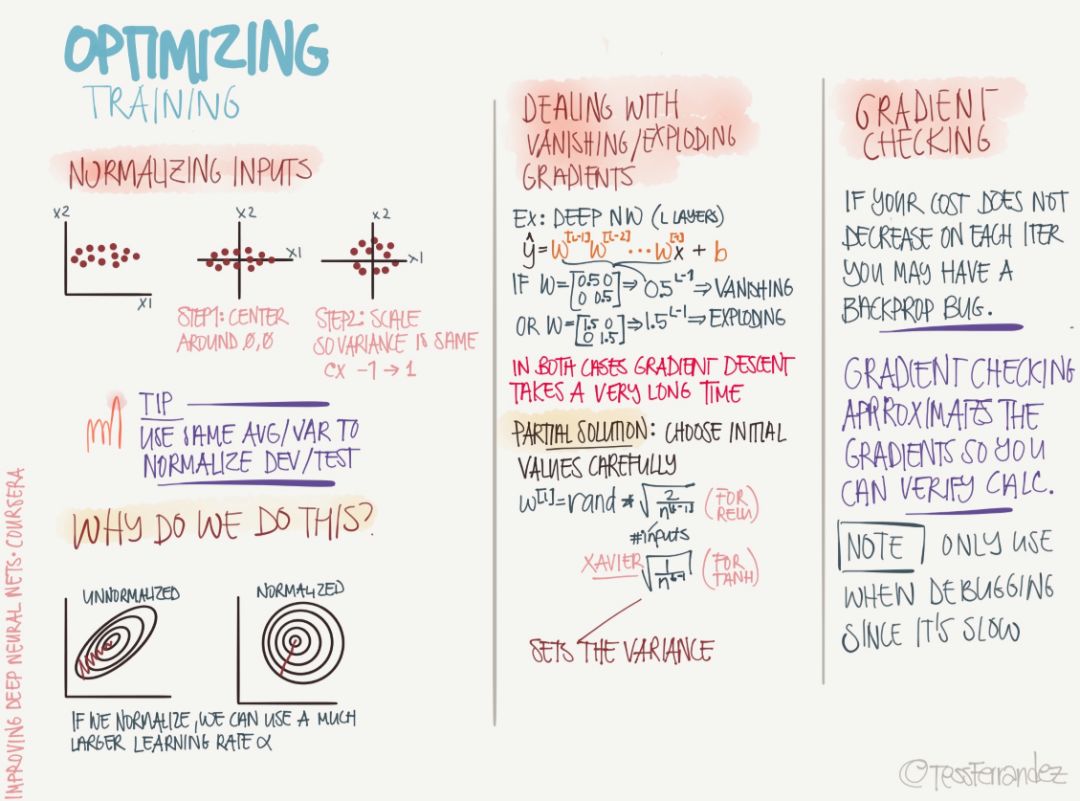
The above shows the problems that often occur with optimization and the required operations. First, before performing the optimization, we need to normalize the input data, and the constants (means and variances) normalized between the development set and the test set are the same as the training set. The above diagram also shows the reason for the normalization, because if the magnitude difference between the features is too large, then the surface of the loss function is a narrow ellipse, and the gradient descent or steepest descent method will be due to the phenomenon of “sawtoothâ€. It is difficult to converge, so normalizing to a circle helps to reduce oscillations in the descending direction.
The problem of the disappearance of gradients and gradient explosions is also a very common phenomenon. "Gradient disappearance" refers to the phenomenon that the gradient exponent of the parameter decreases exponentially as the depth of the network increases. The small gradient means that the parameters change very slowly, which makes the learning process stagnation. Gradient explosion refers to the continuous accumulation of large error gradients in the neural network training process, resulting in a large update of model weights. In extreme cases, the weights become so large that the NaN value appears.
Gradient tests may now be used sparingly because we only need to call the optimizer to perform the optimization algorithm on the TensorFlow or other framework. Gradient testing is generally a numerical method that calculates the approximate derivative and propagates it, so it can test whether or not the gradient we calculate based on the analytical formula is correct.
The following are the specific optimization algorithms, including the most basic small batches of stochastic gradient descent, momentum-based stochastic gradient descent, and adaptive learning rate algorithms such as RMSProp.
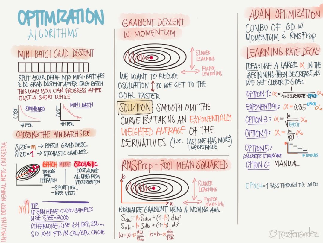
Small batches of stochastic gradient descent (typically SGD refers to this) use a batch of data to update parameters, thus greatly reducing the amount of computation required for an iteration. This method reduces the variance of the updated parameters, making the convergence process more stable; it can also use highly optimized matrix operators in the popular deep learning framework to efficiently find the gradient of each small batch of data. Usually a small batch of data contains between 50 and 256 samples, but it will vary for different purposes.
Momentum strategies are designed to accelerate the learning process of SGD, especially in the case of higher curvature. In general, the momentum algorithm uses the exponentially decaying sliding average of the previous gradient to correct in that direction to better utilize the historical gradient information. The algorithm introduces the variable v as the speed vector for the parameter to move continuously in the parameter space, and the speed can generally be set as the exponentially decaying sliding average of the negative gradient.
The adaptive learning rate algorithms such as RMSProp and Adam described later in the above figure are our most common optimization methods. The RMSProp algorithm (Hinton, 2012) modifies AdaGrad to perform better in non-convex cases, it changes the gradient accumulation to an exponentially weighted moving average, and discards the more distant historical gradient information. RMSProp is the optimization algorithm proposed by Hinton in the open class. Actually, it can be regarded as a special case of AdaDelta. However, it has been proved that RMSProp has very good performance, and it is currently widely used in deep learning.
The Adam algorithm also takes advantage of the AdaGrad and RMSProp algorithms. Adam not only computes the adaptive parameter learning rate based on the first-order moment average as in the RMSProp algorithm, it also makes full use of the gradient second-harmonic mean (ie, there is an uncentered variance).
8 Hyper-parameters
The following is an information diagram that introduces hyperparameters. It plays an important role in neural networks because they can directly improve the performance of the model.
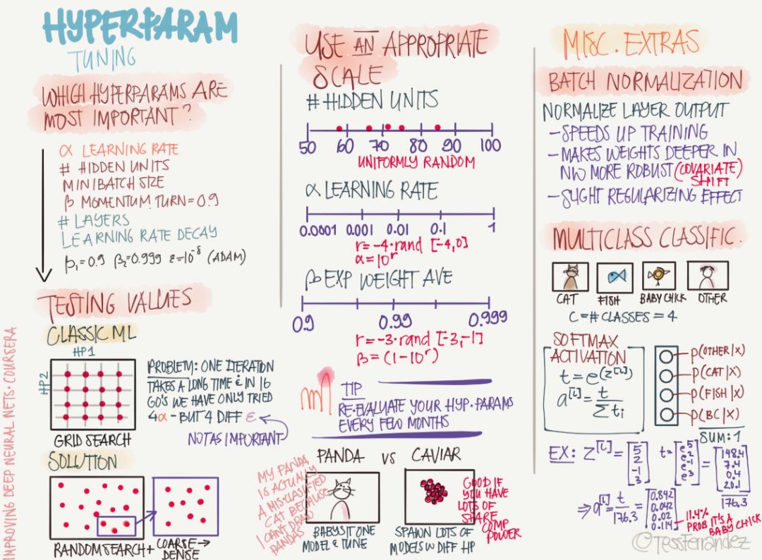
It is well known that hyperparameters such as learning rate, number of hidden units in neural network, batch size, number of levels, and regularization coefficient can directly affect the performance of the model, and how to adjust it becomes very important. At present, the most common is manual tuning. Developers will choose “reasonable†hyperparameters based on their own modeling experience, and then make some minor adjustments based on model performance. However, automation parameters such as stochastic processes or Bayesian optimization still require a very large amount of computation, and the efficiency is relatively low. However, recent advances in searching for hyperparameters using methods such as reinforcement learning, genetic algorithms, and neural networks have made great progress. Researchers are looking for an efficient and accurate method.
The current hyperparametric search methods are:
Rely on experience: Listen to your instincts, set the parameters that you feel right in and see if it works, and keep trying until you get tired.
Grid Search: Let the computer try some values ​​that are evenly distributed within a certain range.
Random search: Let the computer try some random values ​​and see if they work.
Bayesian optimization: using tools like MATLAB bayesopt to automatically pick the best parameters - the result is that Bayesian optimization has more hyperparameters than your own machine learning algorithms, and it doesn't feel like falling back to relying on experience and grids. Search methods go up.
Because of limited space, the following presentation will only briefly introduce the information map, I believe they are very helpful to all readers.
9 Structured Machine Learning Process
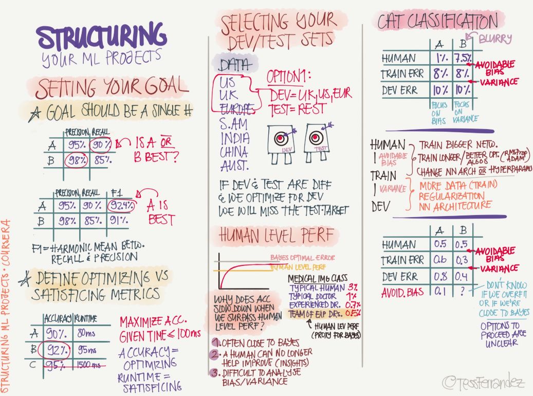
We need to set up our machine learning system according to the process or structure. First we need to set the goal of the model, for example, what its expected performance is and what the measurement method is. Then segment the training, development, and test sets and anticipate the level of optimization that may be reached. Afterwards, the model is built and trained. After the development set and the test set are verified, they can be used to infer.
10 Error Analysis
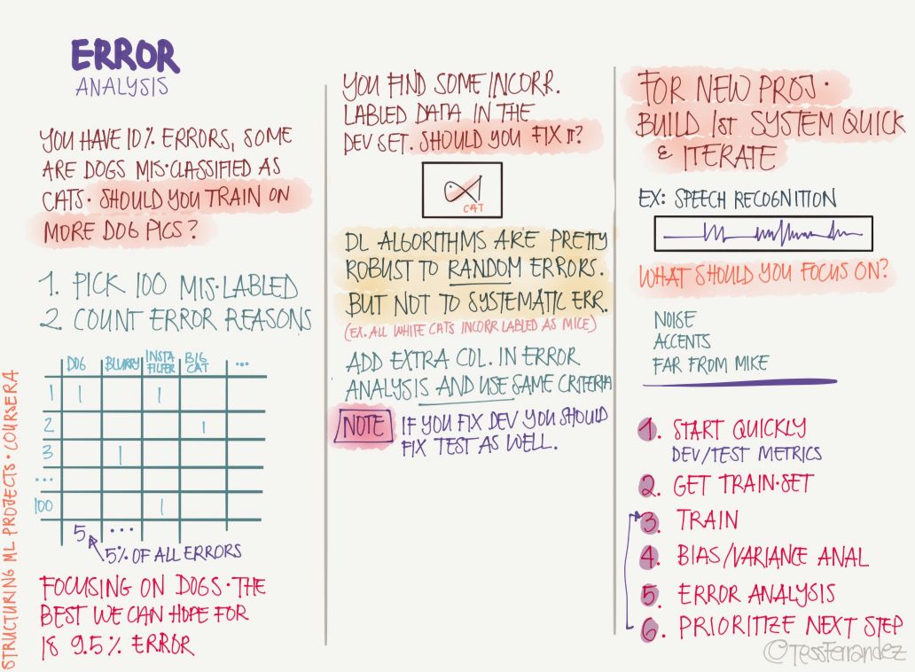
After completing the training, we can analyze the source of the error and improve performance, including the discovery of incorrect labels, incorrect loss functions, and so on.
11 Training Sets, Development Sets, and Test Sets
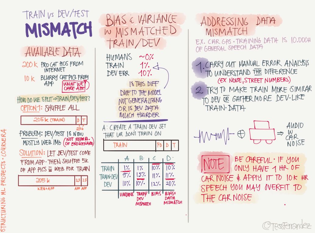
The diagram above shows where the three partitioned datasets and their performances need to be noticed, that is, if they have different correct rates, how can we correct these "differences?" For example, the accuracy of the training set is significantly higher than that of the validation set and the test set, indicating that the model is over-fitted. The accuracy of the three data sets is significantly lower than the acceptable level may be due to under-fitting.
12 Other learning methods
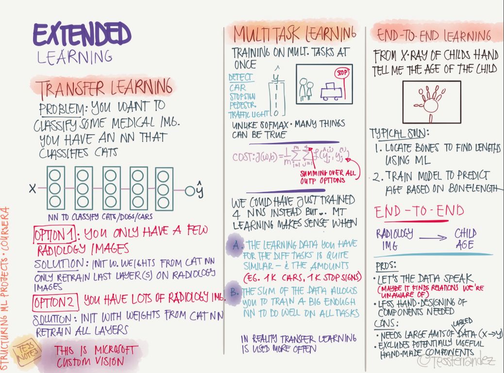
Machine learning and deep learning certainly not only supervise learning methods, but also include transfer learning, multi-task learning and end-to-end learning.
Convolutional network
13 Convolutional Neural Network Basics
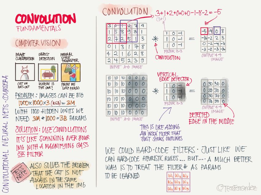
The volume of data involved in computer vision tasks is particularly large. There are thousands of data points for an image, not to mention resolution images and video. At this time, when the network is fully connected, the number of parameters is too large. Therefore, a convolutional neural network (CNN) is used instead. The number of parameters can be greatly reduced. The working principle of CNN is like scanning the entire image with filters that detect specific features, extracting features, and combining layer by layer into increasingly complex features. This "scanning" mode of operation gives it good parameter sharing characteristics so that it can detect the same target (translational symmetry) at different locations.
The detection feature corresponding to the convolution kernel can be easily judged from the distribution of its parameters. For example, the convolution kernel whose weight is reduced from left to right can detect the boundary of black and white vertical stripes, and display the characteristics of the middle bright and dark sides. The specific relative bright and dark results depend on the relative relationship between the image pixel distribution and the convolution kernel. Convolutional kernel weights can be hard-coded directly, but in order to adapt the same architecture to different tasks, it is better to train through the convolution kernel weights.
The main parameters of the convolution operation:
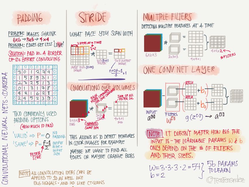
Padding: direct convolution operation will make the feature map getting smaller and smaller, the padding operation will add 0 pixel value edge around the image, make the convolution after the feature map size and the original image (length and width, excluding the channel The number) is the same.
Two commonly used options are: “VALIDâ€, no padding is performed; “SAME†makes the length and width of the output feature map the same as the original image.
Stride: The size of the step between two convolution operations.
A convolutional layer can have multiple convolution kernels. The result of each convolution kernel operation is a channel. The feature maps of each channel have the same length and width and can be stacked to form a multi-channel feature map as the next volume. Stacked input.
Deep convolutional neural network architecture:
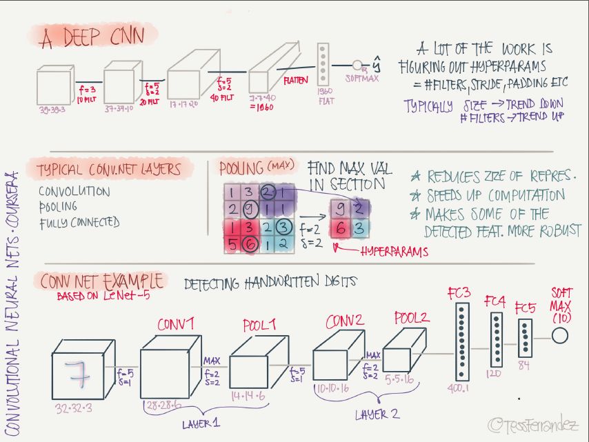
The architecture of deep convolutional neural networks is mainly multi-level stacking of convolutional layers and pooled layers, and finally the full-connection layer performs classification. The main role of the pooling layer is to reduce the size of feature maps, thereby reducing the number of parameters and speeding up calculations, making their target detection performance more robust.
14 Classic Convolutional Neural Networks
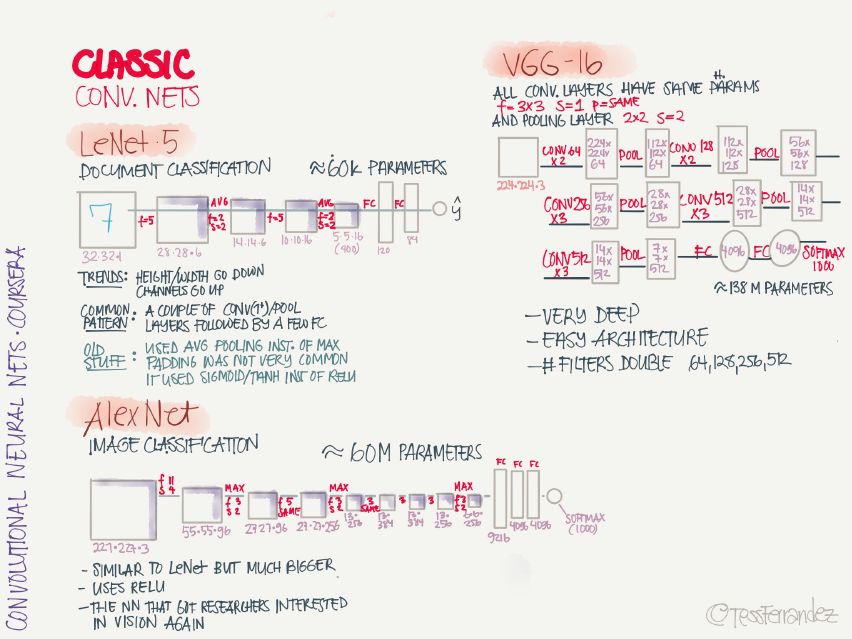
LeNet 5: handwriting recognition classification network, this is the first convolutional neural network proposed by Yann LeCun.
AlexNet: Image classification network, introducing the ReLU activation function on CNN for the first time.
VGG-16: Image classification network, deeper.
15 Special Convolutional Neural Networks
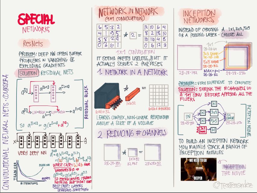
ResNet: The introduction of residual connections to mitigate the gradient disappearance and gradient explosions can train very deep networks.
Network in Network: Using a 1x1 convolution kernel, the convolution operation can be made into a form similar to a fully connected network, and the number of channels in the feature map can also be reduced, thereby reducing the number of parameters.
Inception Network: Using parallel operations of multiple sizes of convolution kernels and stacking into multiple channels, it can capture features of various sizes, but the disadvantage is that the amount of computation is too large and the number of channels can be reduced by 1×1 convolution.
16 Practice Suggestions

Use open source implementations: It is very difficult to implement from scratch, and use other people's implementations to quickly explore more complex and interesting tasks.
Data enhancement: Through the operation of mirroring, random cropping, rotation, and color change of the original image, the training data volume and diversity are increased.
Migration learning: When there is too little training data for the current task, fully trained models can be fine-tuned with a small amount of data to achieve good enough performance.
Good performance in benchmarks and contests: Use model integration, use the average results of multiple model outputs; during the test phase, crop the images into multiple copies and test them separately, and average the test results.
17 Target Detection Algorithm
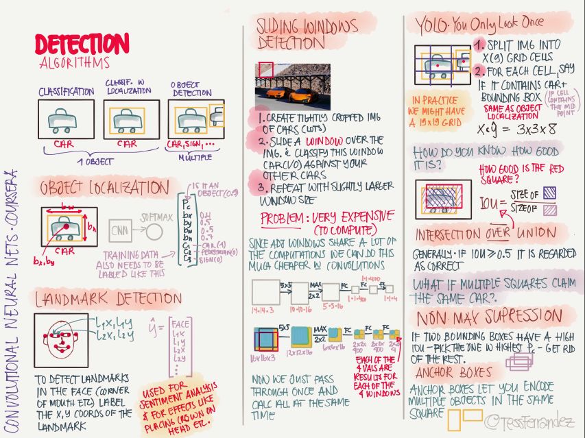
Target detection uses the bounding box to detect the position of objects in the image. Faster R-CNN, R-FCN, and SSD are the three most optimal and most widely used target detection models. The above figure also shows the basic process of YOLO.
18 Face Recognition
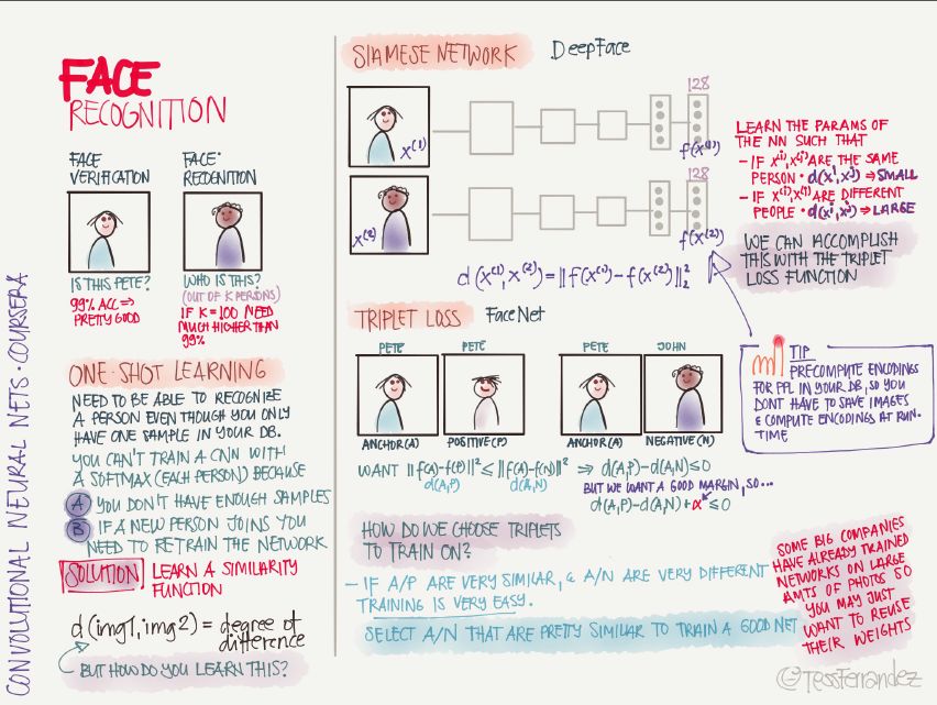
There are two major types of face recognition applications: face verification (bisection classification) and face recognition (multiple person classification).
When the sample size is insufficient, or when new samples are added, one-shot learning is required. The solution is to learn the similarity function, that is, determine the similarity of the two images. For example, when learning face recognition in the Siamese Network, it is to use the output of two networks to reduce the difference between the two outputs of the same person and increase the difference between the two outputs of different people.
19 style migration
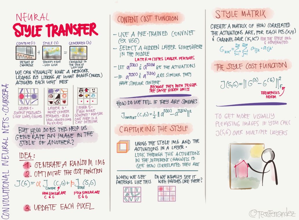
Style migration is a hot topic, it will give people a fresh look. For example, if you have a graph, then apply the style features of another graph to this graph. For example, you can modify your image with the style of a famous painter or a pair of famous paintings, so we can obtain unique style works.
Circular network
20 Recurrent Neural Network Basics
As shown above, serial problems such as named entity recognition occupy a large proportion in real life, while traditional machine learning algorithms such as Hidden Markov Chain can only make strong assumptions and deal with partial sequence problems. But recently, the recurrent neural network has a very big breakthrough on these issues. The structure of the hidden state of RNN is formed into a memory in the form of a loop. The state of the hidden layer at each moment depends on its past state. This structure makes it possible to save the RNN. , remember and deal with long-term past complex signals.
A Recurrent Neural Network (RNN) can learn features and long-term dependencies from sequence and timing data. The RNN has a stack of non-linear cells in which at least one connection between the cells forms a directed loop. A trained RNN can model any dynamic system; however, training RNNs is primarily influenced by long-term learning problems.
The following shows the applications, problems, and variants of RNN:
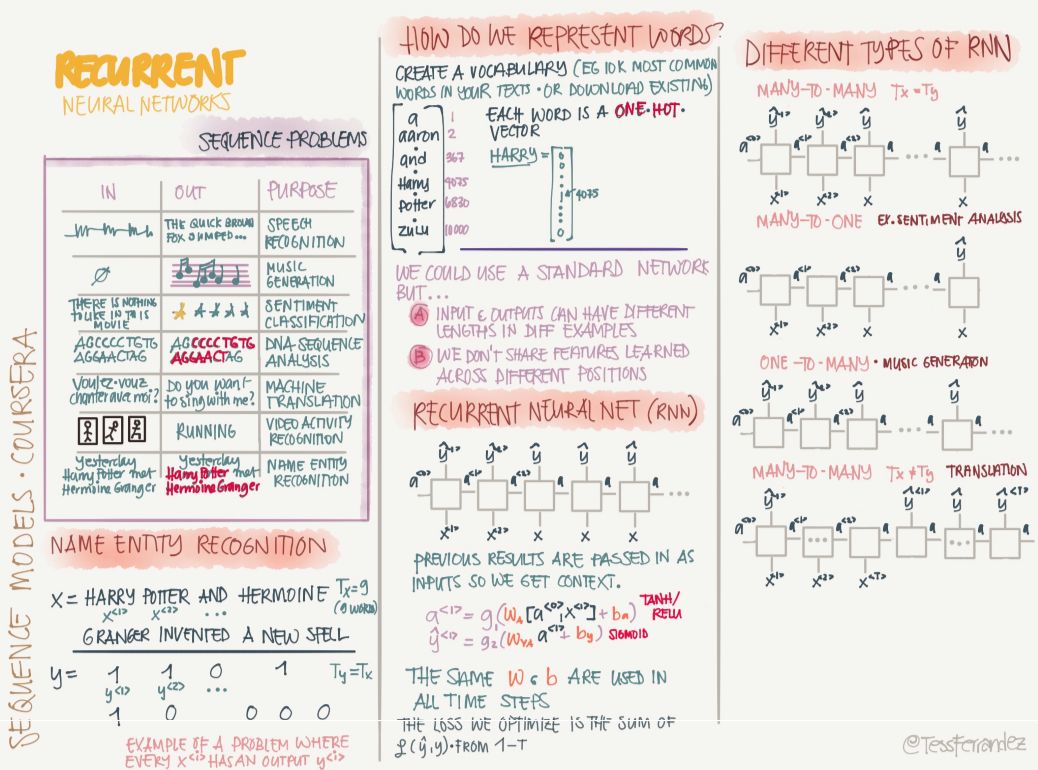
The circulatory neural network has a very powerful power in the sequence of problems such as language modeling, but at the same time it also has a serious gradient disappearance problem. Therefore, gating-based RNNs such as LSTM and GRU have great potential. They use gated mechanisms to retain or forget the information of previous time steps and form memories for the current calculation process.
21 Characterization in NLP

Word embedding is very important in natural language processing because no matter what task is performed, it is necessary to represent the word. The above figure shows the method of word embedding. We can map the vocabulary to a 200 or 300-dimensional vector, which greatly reduces the space for the token. In addition, this method of word representation can also represent the semantics of words, because words with similar meanings are similar in the embedding space.
In addition to the above-mentioned Skip Grams, the following also shows a common way of learning word embedding:
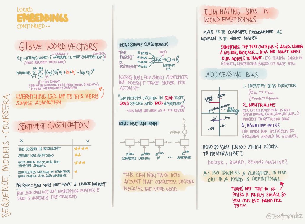
The GloVe word vector is a very common word vector learning method. The word representation it learns can be further used for tasks such as statement classification.
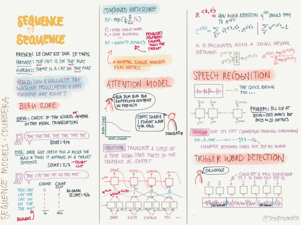
22 Sequence to Sequence

The most used method of sequence-to-sequence is the encoder decoder frame, and other modules such as beam search.
The encoder decoder architecture plus attention mechanisms can solve a very large number of natural language processing problems. The BLEU scores and attention mechanisms are described below. They are indispensable parts in the architecture and evaluation of machine translation.
The above is all the information maps of Wu Enda's deep learning special courses. Since they contain more information, we have only introduced some of them, and many of them are just simple ones. Therefore, it is best for all readers to download this information map and to gradually understand and optimize later in the learning process.
Multi function remote manual pulse generator for control of all axes.
Manual Sensor,Miniature Optical Kit Encoder,Rotary Encoder With Led Ring,Optical Quadrature Encoder
Yuheng Optics Co., Ltd.(Changchun) , https://www.yhenoptics.com