Lei Feng network press: This article translator Liu Xiangyu, Zhongtong soft development engineers, concerned about machine learning, neural networks, pattern recognition.
1. The need of distributed representationsIn a lecture started by Yoshua Bengio, he said, "This is the slide I will focus on." The following figure is this slide:
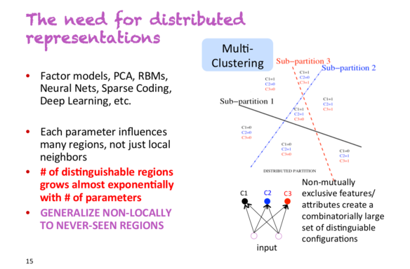
Suppose you have a classifier that needs to classify people as male or female, wear glasses or not wear glasses, high or low. If you use a non-distributed representation, you are dealing with 222 = 8 people. To train high-precision classifiers, you need to collect enough training data for these 8 categories. However, if you use a distributed representation, each attribute will appear in other different dimensions. This means that even if the classifier does not meet the tall man wearing glasses, it can successfully identify them because it learns to learn to recognize gender separately from other samples, whether to wear glasses or not and height.
2, local minimum is not a problem in the high dimensionYoshua Bengio's team found through experiments that there is no local minimum when optimizing high-dimensional neural network parameters. In contrast, there are saddle points in some dimensions, which are locally minimal but not globally minimal. This means that training at these points will slow down until the network knows how to leave these points, but we are willing to wait long enough for the network to find ways.
The following figure shows the vibrations of the two states during network training: near the saddle point and leaving the saddle point.
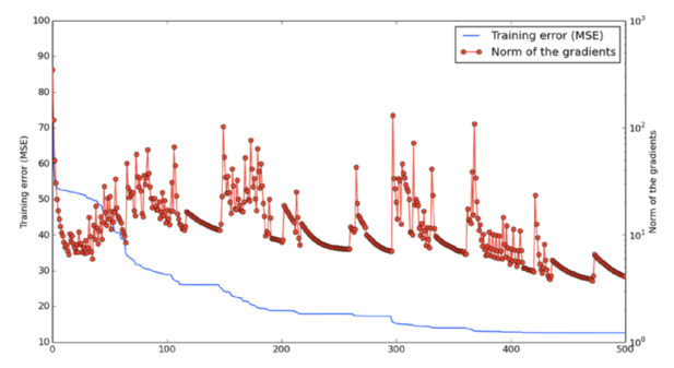
Given a specified dimension, the small probability p represents the probability that the point is a local minimum, but not the global minimum in this dimension. The point in the 1000-dimensional space is not a local minimum probability and it will be, this is a very small value. However, in some dimensions, the local minimum probability of this point is actually higher. And when we get the minimum value in multiple dimensions at the same time, training may stop until we find the right direction.
In addition, the probability p increases as the loss function approaches the global minimum. This means that if we find a true local minimum, then it will be very close to the global minimum, and this difference is irrelevant.
3, derivative function, derivative function, derivative functionLeon Bottou lists some useful tables about activation functions, loss functions, and their corresponding derivatives. I put them first here for later use.
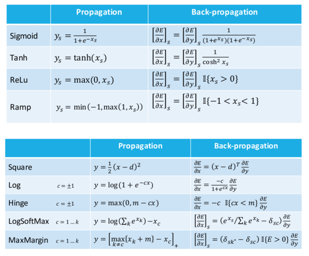
Update: According to the comment, the minimum and maximum functions in the slope formula should be swapped.
4, weight initialization strategyThe current weight initialization strategy recommended in neural networks is to normalize values ​​to the range [-b,b], where b is:
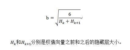
Recommended by Hugo Larochelle, published by Glorot and Bengio (2010).
5, neural network training skillsHugo Larochelle gives some practical advice:
Normalized real-valued data. Subtract the average and divide by the standard deviation.
Reduce the learning rate in the training process.
Updating the data using small batches will make the gradient more stable.
Use momentum through the stagnation period.
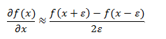
6, gradient detectionIf you manually implement the back-propagation algorithm but it doesn't work, there is a 99% chance of a bug in the gradient calculation. Then use gradient detection to locate the problem. The main idea is to use the definition of a gradient: if we increase the weight value slightly, the error of the model will change.
There is a more detailed explanation here: Gradient checking and advanced optimization.
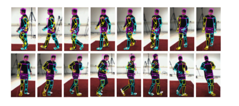
7, motion trackingHuman body motion tracking can achieve very high accuracy. The following figure is an example from the paper Dynamical Binary Latent Variable Models for 3D Human Pose Tracking published by Graham Taylor et al. (2010). This method uses a conditionally constrained Boltzmann machine.
Chris Manning and Richard Socher have invested a lot of effort to develop a combination model that combines neural embedding with more traditional analysis methods. This reached the limit in the paper Recursive Neural Tensor Network, which uses the interaction of addition and multiplication to combine word sense and parse trees.
Then, the model was defeated by the Paragraph vector (Le and Mikolov, 2014) (with a considerable gap), and the Paragraph vector had no knowledge of the sentence structure and syntax. Chris Manning called this result "a failure to create a 'good' combination vector."
However, more and more work results using the syntax parse tree have changed that result. Irsoy and Cardie (NIPS, 2014) successfully defeated the Paragraph vector using a deeper network in multiple dimensions. Finally, Tai et al. (ACL, 2015) combined the LSTM network with the parsing tree to further improve the results.
The accuracy of the results of these models on the Stanford Type 5 sentiment dataset is as follows:
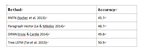
From a current point of view, using a parsed tree model is superior to a simple method. I am curious about when the next non-grammar-based method will appear and how it will promote the game. After all, the goal of many neural models is not to discard the underlying grammar, but to implicitly capture it in the same network.
9, distributed and distributedChris Manning himself clarified the difference between these two words.
Distributed : The level of continuous activation in several elements. Such as dense vocabulary embedding, rather than 1-hot vector.
Distributive : Indicates the context of use. Word2vec is distributed, and when we use the lexical context to model semantics, the count-based vocabulary vectors are also distributed.
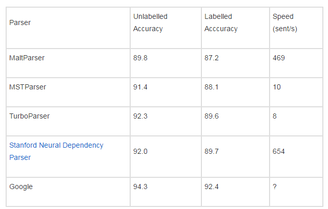
10. Dependency status analysisPenn Treebank dependency analyzer comparison:
 Â Â
 Â
The final result was derived from Google's "Extract all stops" and used massive amounts of data to train the Stanford NeuroGram Parser.
11, Theano
I knew Theano before, but I learned more in summer school. And it's really great.
Since Theano originated in Montreal, developers who consult Theano directly can be useful.
Most of the information about it can be found online, in the form of an interactive Python tutorial.
12, Nvidia DigitsNvidia has a toolkit called Digits that trains and visualizes complex neural network models without writing any code. And they are selling DevBox, a custom machine that can run Digits and other deep learning software (Theano, Caffe, etc.). It has 4 Titan X GPUs and is currently priced at $15,000.
13, FuelFuel is a tool for managing dataset iterations. It can divide a dataset into smaller parts, perform shuffle operations, and perform various preprocessing steps. There are preset features for some established datasets, such as MNIST, CIFAR-10, and Google's one billion lexical corpus. It is mainly used in conjunction with Blocks, which is a tool for using Theano to simplify the network structure.
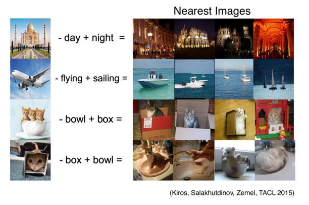
14. Multi-model linguisticsRemember "King - Male + Female = Queen"? In fact, pictures can be treated as such (Kiros et al., 2015).
When we move to the point, we can estimate the value of the function at the new position by calculating the derivative function. We will use the Taylor series approximation:

Similarly, when we update the parameters, we can estimate the loss function:

Where g is the derivative of θ and H is the second-order Hessian derivative of θ.
This is a second-order Taylor approximation, but we can increase accuracy by using higher order derivatives.
16, calculated intensityAdam Coates proposed a strategy for analyzing the speed of matrix operations on GPUs. This is a simplified model that can display the time spent reading memory or performing calculations. Assuming you can calculate these two values ​​at the same time, we can know that that part takes more time.
Suppose we multiply the matrix by a vector:
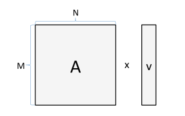
If M=1024, N=512, then the number of bytes we need to read and store is:
4 bytes × (1024×512+512+1024)=2.1e6 bytes
The number of calculations is:
2×1024×512=1e6 FLOPs
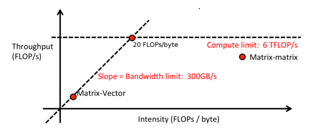
If we have a GPU with a block size of 6TFLOP/s and a bandwidth of 300GB/s, then the total running time is:
Max{2.1e6 bytes/(300e9 bytes/s), 1e6 FLOPs/(6e12 FLOP/s)}=max{7μs, 0.16μs}
This means that the bottleneck of the process is the 7μs consumed by copying from memory or writing to memory, and using a faster GPU will not increase the speed. As you might guess, this situation will improve when the matrix/vector is large when performing matrix-matrix operations.
Adam also gives an algorithm for calculating the operating intensity:
Intensity = (arithmetic operation)/(byte load or number of stores)
In previous scenarios, the intensity was like this:
Intensity = (1e6 FLOPs)/(2.1e6 bytes) = 0.5FLOPs/bytes
Low intensity means that the system is hampered by the size of the memory, and high intensity means being hampered by the speed of the GPU. This can be visualized to determine which aspects should be improved to improve overall system speed and where the best point can be observed.
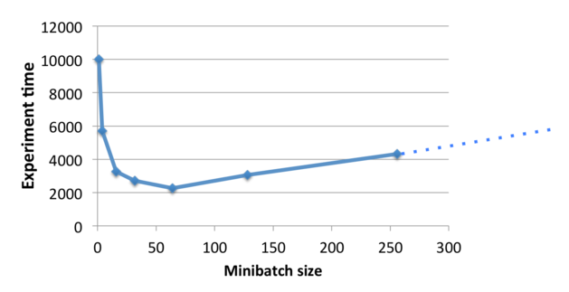
Continuing to talk about computational strength, one way to increase network strength (by calculation rather than memory limitation) is to divide the data into small batches. This avoids some memory operations and the GPU is also good at parallel processing of large matrix calculations.
However, increasing the size of the batch may have an effect on the training algorithm, and the merger takes more time. It is important to find a good balance to get the best results in the shortest possible time.
According to recent information, neural networks can be easily teased against the sample. In the following case, the pictures on the left are correctly classified as goldfish. However, if we join the noise pattern of the middle picture, we get the picture on the right, and the classifier thinks this is a picture of a daisy. Image from Andrej KarPathy's blog "Breaking Linear Classifiers on ImageNet", you can learn more about that.
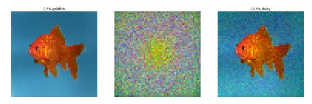
The noise pattern is not randomly selected, but is used to tease the network through meticulous calculations. But the problem persists: the image on the right is obviously a goldfish rather than a daisy.
Obviously, like integrated models, multi-saccade voting and unsupervised pre-training strategies cannot solve this loophole. Using a high degree of regularization will help, but it will affect the accuracy of judging non-noise images.
Ian Goodfellow proposed the idea of ​​training these countermeasures. They can be automatically generated and added to the training set. The following results show that in addition to helping the counter sample, this also improves the accuracy of the original sample.
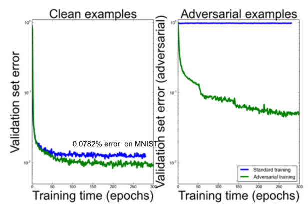
Finally, we can further improve the results by penalizing the KL divergence between the original predicted distribution and the predicted distribution on the counter sample. This will optimize the network to make it more robust and able to predict similar class distributions for similar (counter) images.
19. All things are language modelingPhil Blunsom suggested that almost all NLPs can be built into language models. We can do this by connecting the output with the input and trying to predict the probability of the entire sequence.
translation:
P(Les chiens aiment les os || Dogs love bones)
Q&A:
P(What do dogs love? || bones .)
dialogue:
P(How are you? || Fine thanks. And you?)
The latter two must be based on understanding what is known in the world. The second part may not even be a word, but it may also be a tag or a structured output, such as a dependency.
20, SMT difficult to beginWhen Frederick Jelinek and his team at IBM submitted a paper on one of the first batches of statistical machine translation in 1988, they went to the following anonymous review:
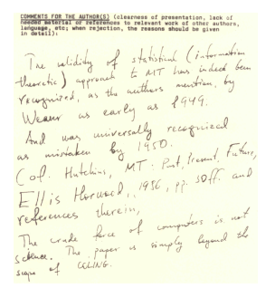
As the author mentioned, as early as 1949 Weaver affirmed the effectiveness of statistical (informational) methods for machine translation. It was generally considered wrong in 1950 (see Hutchins, MT – Past, Present, Future, Ellis Horwood, 1986, p. 30ff and references). Violence in computers is not science. The paper is beyond the scope of COLING.
21. Status of Neural Machine TranslationObviously, a very simple neural network model can produce surprisingly good results. The following figure is a slide by Phil Blunsom to translate Chinese into English:
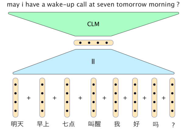
In this model, the Kanji vectors simply add together to form a statement vector. The decoder includes a conditional language model that combines the statement vector with the vectors from the two most recently generated English words and then generates the next word in the translation.
However, neural models still do not maximize the performance of traditional machine translation systems. But they are already quite close. Results of Sutskever et al. (2014) in "Sequence to Sequence Learning with Neural Networks":
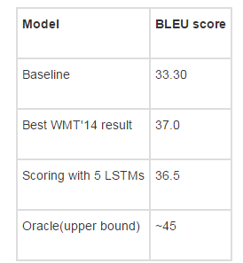
Update: @stanfordnlp pointed out that some recent results show that the neural model will really maximize the performance of traditional machine translation systems. View the paper "Effective Approaches to Attention-based Neural Machine Translation" (Luong et al., 2015)
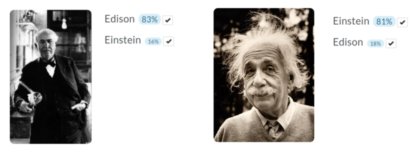
Richard Socher demonstrated examples of image classification for great people. You can upload images for training. I trained a classifier that can recognize Edison and Einstein (can't find enough Tesla personal photos). Each class has 5 sample pictures and tests the output image for each class. It seems to work well.
Mark Schmidt gives two reports on numerical optimization in different situations.
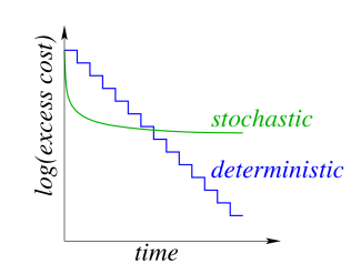
In the deterministic gradient method, we calculate the gradient over the entire data set and then update it. The iterative cost has a linear relationship with the data set size.
In the stochastic gradient method, we calculate the gradient on one data point and then update it. Iteration costs are independent of the data set size.
Each iteration in a random gradient descent is much faster, but it usually requires more iterations to train the network, as shown in the following figure:
In order to achieve the best effect of both, we can use batch processing. Specifically, we can perform a random gradient descent on the data set to quickly reach the right part and then start increasing the batch size. The gradient error decreases as the batch size increases, but the final iteration cost size will still depend on the data set size.
The stochastic mean gradient (SAG) can avoid this situation, with only one gradient per iteration, resulting in a linear convergence rate. Unfortunately, this is not feasible for large neural networks because they need to remember the gradient update of each data point, which will consume a lot of memory. The random variance reduction gradient (SVRG) can reduce this memory consumption situation, and each iteration (plus occasional full passes) requires only two gradient calculations.
Mark said that one of his students implemented various optimization methods (AdaGrad, momentum, SAG, etc.). When asked what method he would use in a black box neural network system, the student gave two methods: Streaming SVRG (Frostig et al., 2015), and a method they had not yet published.
24. Theano analysisIf you assign "profile=true" to THEANO_FLAGS, it will analyze your program and then display the time spent on each operation. It is helpful to find performance bottlenecks.
25, adversarial network frameworkFollowing Ian Goodfellow's speech on confrontational samples, Yoshua Bengio talked about the case of competing with two systems.
System D is a set of discriminative systems whose purpose is to classify real data and artificially generated data.
System G is a set of generation system that attempts to generate data that can allow system D to misclassify it into real data.
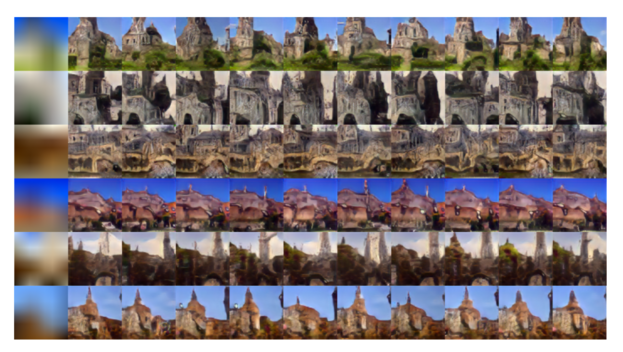
When we train a system, the other system must also become better. This works well in experiments, but the step size must be kept small enough so that System D can be even faster on G. Here are some examples of "Deep Generative Image Models using a Laplacian Pyramid of Adversarial Networks" - a more advanced version of this model that attempts to generate images of churches.
The arXiv number contains the year and month of submission of the paper, followed by the serial number. For example, paper 1508.03854 represents the number 3854 paper submitted in August 2015. Glad to know this.
Via graphic
Lei Feng network (search "Lei Feng network" public concern) Note: This article is authorized by the CSDN authorized Lei Feng network, if you need to reprint please contact the authorization.
Toroidal Transformer,Toroidal Transformer Audio,Diy Toroidal Transformer,Toroidal Current Voltage Transformer
Guang Er Zhong(Zhaoqing)Electronics Co., Ltd , https://www.geztransformer.com